More Binary Heaps and Heap Sort Algorithm


Hello people…! In this post I will talk about the Binary Heap implemented using structures and not arrays. This is post is the successor to my previous post on Binary Heaps. Using arrays to code Binary Heaps is very comfortable for the programmer. But it is not fit for the day-to-day applications. This is because the Binary Heap is used to implement the Priority Queue and it is meant to grow, not stay of fixed size. But given that it is meant to grow, we cannot use STL Vector for this. This is because the Vector keeps reallocating memory as it grows. So, it is slow. Here we will learn the proper structure based implementation of the Binary Heaps.

Now, currently we have the knowledge of the Binary Heap, its structure, working and other properties. But we implemented this using arrays. Now if we were to implement using a structure, there is one challenge that we will face. That is to ensure the Structural Property of the heap. Why? For insertion into an array, we created a node at the end which itself ensured the Structural Property is not violated and then we bubbled upwards to ensure that the Heap Property is not violated at any point. In the array, we knew exactly where we are supposed to insert the node. But in a tree coded using structures how will you find where to insert the new element such that the tree remains a complete binary tree..? The same goes when we want to delete the root. How do we know where the last node is. For this, we will use the binary representation of the size of the heap to traverse to the location we want.

Size does matter !

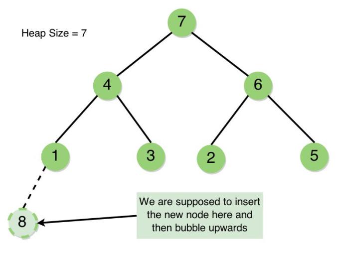
While inserting itself we could keep a track of the heap size. So, this takes constant time. While inserting, we must search for the appropriate location. For this, we will convert the size into its binary representation and begin the traversal from the root. How? Keep reading the bits of the binary representation you just generated, if you encounter ‘0’ go to the left child of the parent, if it is a ‘1’ go to the right child of the parent. I know it sounds really weird, but that’s the best thing we can do. Let’s take up an example to understand this better. Consider the Binary Heap below –

BinaryHeaps1

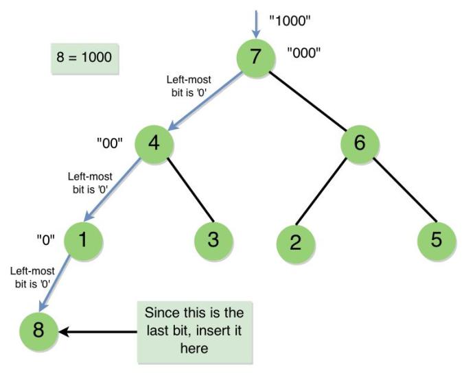
Now consider the binary representation of the number (HeapSize + 1) = 8, which is “1000”. We omit the first bit (left-to-right) because that bit says “come to the root”.

  • The Binary String left is “000”. The leftmost bit is ‘0’. So, go to the Left Child. You come to Node 4.
  • The Binary String left is “00”. The leftmost bit is ‘0’. So, go to the Left Child. You come to Node 1.
  • The Binary String left is “0”. There is only one bit left. This bit doesn’t tell you to “go left” or “go right”, it tells you to “insert it to left” or “insert it to right”. As this bit is “0”, we place the new node as the left child of Node 1.

This is how you must use the binary representation of the (HeapSize + 1) to get to the location you want to insert the node. This is process is depicted in the sketch below –

BinaryHeaps2

Every time you insert a node, you will go all the way down the tree, you will not perform any insertions in the middle, so the traversal always takes O(log n), once inserted, you travel up, ensuring that the heap property holds good, so you have to travel all the way up again, so it is another O(log n) operation. So, the over all process takes O(log n), which is same as in the case of an array implementation.

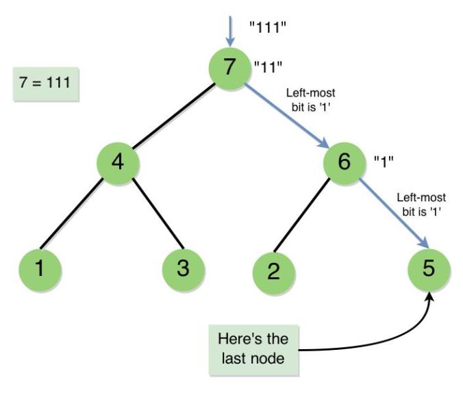
But for deletion, we are supposed to find something else. We are supposed to find out the last node. In the sketch above, before the insertion of 8, we are supposed to somehow find out that the last node is Node 5. There are a couple of methods by which we can accomplish this –

  1. BFS or DFS – By using the Breadth First Search or the Depth First Search we can find out which is the last node in the Binary Heap by searching the whole tree for a node at the maximum depth which is encountered as last as possible. The time complexity of BFS and DFS is O(|E| + |V|). We would have N vertices and what about the number the edges? We would have N – 1 edges, because every node is pointed by a child pointer, except the root. So, the overall complexity becomes O(N + N), which is O(N).
  2. Binary Traversal – This is the same traversal as we did in the case of Insertion. I just called it Binary Traversal. But the method which we discussed about gave us the Node to be inserted but not the last node. Can you think of a way of modifying the procedure such that it would give us the last node directly…? Think about this for a couple of minutes and you will figure out the simple logic behind it. For those who can’t, don’t worry I will discuss it, when I do, try to figure how silly a thing you missed…! The logic is simple, you used the binary representation of (HeapSize + 1) to get to the location where you were supposed to insert a node, if you use the binary representation of (HeapSize) itself for traversal, you will end up at the last node…! Try working out this on paper and you will realise the logic behind it. As, we would traverse the whole tree from root to leaf, this takes O(log N), which is way faster than BFS and DFS which was an O(N) operation. This kind of Binary Traversal is depicted in the sketch below –

BinaryHeaps3

The next thing that we must know about the structure implementation is that unlike the array implementation, where we could construct the heap using build heap procedure, we cannot do that here. The only way to construct the heap from a given collection of numbers is to keep inserting them one-by-one. As we discussed that in insertion, we would have to go all the way down and come up, inserting a node in the structure implementation will be slower than inserting into a heap implemented using arrays.

So, now let us plan what we would be writing as our code. First things first..! The structure of our nodes in the heap would be –

struct node
{
	int value;
	struct node * parent;
	struct node * leftChild;
	struct node * rightChild;
};

Apart from the standard variables that we see in many structure related codes, we would be needing the parent pointer here. This is because, without that, we cannot travel up the tree, which is needed in insertion and deletion.

Heap Sort – If you have understood the concepts of constructing the Binary Heap, finding the Last Node and Extracting maximum element, then Heap Sort becomes obvious. You just have to keep extracting the maximum element and store it in an array or a list. Then, you will have a sorted array. This essentially destroys the entire heap.

Take a break and come back to code the binary heap. If you have already coded the binary search tree or a binary tree before this should be relatively easy for you. If you have not, then this will be challenging, and I’m sure you’ll be proud of your efforts once you have successfully coded this data structure. You will spend 80% of the time debugging your code, and trust me that’s the way programming is done. I can’t discuss the issues that you might encounter while coding but you can always comment them if you need help. Once you are able to code Insertion and Deletion, Heap Sort should be easy. If you get stuck, you can always refer to my code below –

/*
 * Binary Heap using Structures
 * and Heap Sort Algorithm
 *
 * Authored by,
 * Vamsi Sangam
 */

#include <cstdio>
#include <cstdlib>
#include <list>

using namespace std;

struct node
{
	int value;
	struct node * parent;
	struct node * leftChild;
	struct node * rightChild;
};

// Traverses the Heap top-to-bottom once and returns the location
// of the last node. Works on the priciple of traversing a
// Binary Tree by the binary representation of its size.
struct node * findLastNode(struct node * BinaryHeap, int size)
{
	list<int> Stack;

	// Getting the binary
	// representation of the size
	while (size != 0) {
		if (size & 1) {
			Stack.push_front(true);
		} else {
			Stack.push_front(false);
		}

		size = size >> 1;
	}

	// Omit the first bit
	Stack.pop_front();

	struct node * traverse = BinaryHeap;
	bool temp;

	while (Stack.size() != 0) {
		temp = Stack.front();
		Stack.pop_front();

		if (temp) {
			// encountered 1
			// go to rightChild
			traverse = traverse->rightChild;
		} else {
			// encountered 0
			// go to leftChild
			traverse = traverse->leftChild;
		}
	}

	return traverse;
}

// This makes the neccessary adjustments
// after insertion to ensure the validity
// of Heap Property in the Binary Heap
void bubbleUp(struct node * heap)
{
	if (heap->parent == NULL) {
		return;
	}

	if (heap->parent->value < heap->value) {
		// Swap child and parent
		int temp = heap->value;
		heap->value = heap->parent->value;
		heap->parent->value = temp;

		bubbleUp(heap->parent);
	}
}

// The recursive procedure which goes top-to-bottom from the root to the place of
// insertion and inserts the new node with a value 'Value'. Uses binary traversal.
struct node * insertUtil(struct node * BinaryHeap, int value, list<bool> * Stack)
{
	bool temp;

	if ((*Stack).size() == 1) {
		temp = (*Stack).front();
		(*Stack).pop_front();

		if (temp) {
			// create new node as the right child
			BinaryHeap->rightChild = (struct node *) calloc(1, sizeof(struct node));
			BinaryHeap->rightChild->parent = BinaryHeap;
			BinaryHeap = BinaryHeap->rightChild;
			BinaryHeap->value = value;
		} else {
			// create new node as the left child
			BinaryHeap->leftChild = (struct node *) calloc(1, sizeof(struct node));
			BinaryHeap->leftChild->parent = BinaryHeap;
			BinaryHeap = BinaryHeap->leftChild;
			BinaryHeap->value = value;
		}
	} else {
		temp = (*Stack).front();
		(*Stack).pop_front();

		if (temp) {
			// encountered 1
			// go to rightChild
			BinaryHeap = insertUtil(BinaryHeap->rightChild, value, Stack);
		} else {
			// encountered 0
			// go to leftChild
			BinaryHeap = insertUtil(BinaryHeap->leftChild, value, Stack);
		}
	}

	return BinaryHeap;
}

// Inserts a new node into the binary heap and also makes
// the neccessary swaps to ensure Heap Property isn't violated
void insertIntoHeap(struct node * BinaryHeap, int value, list<bool> * Stack)
{
	(*Stack).pop_front(); // Omit the first bit

	// Inserting into Heap and keeping a
	// track of the newly inserted node
	struct node * newNode = insertUtil(BinaryHeap, value, Stack);

	// Bubble the new node up the
	// Heap to ensure validity of
	// the Heap Property
	bubbleUp(newNode);
}

// Allocates memory for the Binary
// Heap thus creates the root node
struct node * getBinaryHeap(int value)
{
	struct node * BinaryHeap = (struct node *) calloc(1, sizeof(struct node));

	BinaryHeap->value = value;

	return BinaryHeap;
}

// A simple utility function
// to aid In-Order Walk
void print(struct node * BinaryHeap)
{
	printf("%d ", BinaryHeap->value);
}

// Prints the nodes of the Binary
// Heap in the In-Order fashion
void inOrderTraversal(struct node * BinaryHeap)
{
	if (BinaryHeap == NULL) {
		return;
	}

	inOrderTraversal(BinaryHeap->leftChild);
	print(BinaryHeap);
	inOrderTraversal(BinaryHeap->rightChild);
}

// The standard recursive Heapify procedure to
// convert a partial heap to a complete heap
// Mainly used by Extract-Max procedure
void heapify(struct node * BinaryHeap)
{
	if (BinaryHeap->leftChild != NULL && BinaryHeap->rightChild != NULL) {
		// both children exist

		if (BinaryHeap->value < BinaryHeap->leftChild->value && BinaryHeap->value < BinaryHeap->rightChild->value) {
			if (BinaryHeap->leftChild->value > BinaryHeap->rightChild->value) {
				// leftChild is greater

				int temp = BinaryHeap->value;
				BinaryHeap->value = BinaryHeap->leftChild->value;
				BinaryHeap->leftChild->value = temp;

				heapify(BinaryHeap->leftChild);
			} else {
				// rightChild is greater

				int temp = BinaryHeap->value;
				BinaryHeap->value = BinaryHeap->rightChild->value;
				BinaryHeap->rightChild->value = temp;

				heapify(BinaryHeap->rightChild);
			}
		} else if (BinaryHeap->value < BinaryHeap->leftChild->value && BinaryHeap->value > BinaryHeap->rightChild->value) {
			// leftChild is greater & rightChild is smaller than parent

			int temp = BinaryHeap->value;
			BinaryHeap->value = BinaryHeap->leftChild->value;
			BinaryHeap->leftChild->value = temp;

			heapify(BinaryHeap->leftChild);
		} else if (BinaryHeap->value > BinaryHeap->leftChild->value && BinaryHeap->value < BinaryHeap->rightChild->value) {
			// rightChild is greater & leftChild is smaller than parent

			int temp = BinaryHeap->value;
			BinaryHeap->value = BinaryHeap->rightChild->value;
			BinaryHeap->rightChild->value = temp;

			heapify(BinaryHeap->rightChild);
		}
	} else if (BinaryHeap->rightChild == NULL && BinaryHeap->leftChild != NULL) {
		// Only the leftChild exists

		if (BinaryHeap->leftChild->value > BinaryHeap->value) {
			// The existing leftChild is greater than parent
			// So swap

			int temp = BinaryHeap->leftChild->value;
			BinaryHeap->leftChild->value = BinaryHeap->value;
			BinaryHeap->value = temp;
		}

		// When we reach here, logically speaking, we have come
		// to the last node in the Binary Heap, so after this
		// we simply return from the function
	}
}

// Returns the root value and deletes it by swapping the root
// node and the last node and then calling heapify on root node
int extractMax(struct node * BinaryHeap, struct node * lastNode)
{
	if (BinaryHeap == NULL) {
		return -1;
	}

	if (BinaryHeap == lastNode) {
		// A corner case where only
		// one node exists

		int max = BinaryHeap->value;

		free(BinaryHeap);

		return max;
	}

	int max = BinaryHeap->value;

	// Swap root node and last node
	int temp = BinaryHeap->value;
	BinaryHeap->value = lastNode->value;
	lastNode->value = temp;

	// Making its parent point to NULL appropriately
	struct node * parent = lastNode->parent;

	if (parent->leftChild == lastNode) {
		parent->leftChild = NULL;
	} else {
		parent->rightChild = NULL;
	}

	// Deleting the lastNode
	free(lastNode);
	heapify(BinaryHeap);	// making adjustments

	return max;
}

// Heap Sort procedure which takes and empyt list 'Sorted List'
// and fills it with the elements in sorted order. Keeps extracting
// the maximum element from the Max Heap until it is empty
void heapSort(struct node * BinaryHeap, list<int> * SortedList, int HeapSize)
{
	struct node * lastNode;
	list<int>::iterator itr;

	while (HeapSize != 0) {
		//getting the lastNode to assist extractMax procedure
		lastNode = findLastNode(BinaryHeap, HeapSize);
		(*SortedList).push_front(extractMax(BinaryHeap, lastNode));
		--HeapSize;
	}
}

int main()
{
	int n;

	printf("Enter the size of input -\n");
	scanf("%d", &n);

	int temp, i, j, HeapSize = 0;
	struct node * BinaryHeap;
	list<bool> Stack;

	printf("\nEnter %d integers -\n", n);

	for (i = 0; i < n; ++i) {
		scanf("%d", &temp);
		++HeapSize;

		if (i == 0) {
			BinaryHeap = getBinaryHeap(temp);
			continue;
		}

		// Clears the Stack before filling it with
		// the Binary Representation of HeapSize
		Stack.clear();
		j = HeapSize;

		while (j != 0) {
			if (j & 1) {
				Stack.push_front(true);
			} else {
				Stack.push_front(false);
			}

			j = j >> 1;
		}

		insertIntoHeap(BinaryHeap, temp, &Stack);
	}

	printf("\nIn Order Traversal - ");
	inOrderTraversal(BinaryHeap);
	printf("\n");

	list<int> SortedList;

	heapSort(BinaryHeap, &SortedList, HeapSize);
	BinaryHeap = NULL;

	list<int>::iterator itr = SortedList.begin();

	printf("\nElements in Sorted order - ");
	while (itr != SortedList.end()) {
		printf("%d ", *itr);
		++itr;
	}
	printf("\n");

	return 0;
}

The code is big and that is how it should be and moreover, it is well commented with information. If you still have doubts regarding the code or any concept, feel free to comment them. I hope my post has helped you to get a complete idea about the Binary Heap. If it did, let me know by commenting…! Keep practising… Happy Coding…! 🙂
You may also like –

More in the Navigation Page ! →

Segment Trees


Hello people…! In this post I will talk about one of the most versatile data structure in competitive programming, the Segment Tree. Almost in every contest that you do in the major coding websites, at least one question is asked which uses a Segment Tree in its solution. This is because it is easy to code, and does some useful operations quickly, in logarithmic time. Segment Trees are used where the problem demands these two queries on a given array arr[1 … n] –

  1. Sum of elements in the range arr[L … R]. Where, 1 <= L <= R <= n.
  2. Updating an element arr[i].

You can think of doing this in the naive approach where you directly operate on the input array itself. You could do the first operation in O(n) time by running a loop calculate the sum. The second operation could be done in O(1) time, because, it’s only simply updating. This is good if the number of sum queries asked are very less and the update queries are more.

The next best thing you could think of is, Prefix Sum Array. The Prefix Sum Array is an array where the element arr[i] holds the sum of values from arr[1] to arr[i]. You can construct the Prefix Sum Array in O(n) time and solve the first query in O(1) time. Prefix Sum Array is one of my favourite techniques to find out the sum in a given range. But the update query takes O(n) time. If you want to update the ith element, you’d have to update all the elements from i to n, which takes O(n) in the worst case.

How about doing both of them in O(log n) time…? That’s really quick..! This is the speciality of the Segment Tree. We can get the sum query and the update query done in logarithmic time. The Segment Tree works on the principle of partial sums. If you have read my post on Fenwick Trees (or) Binary Indexed Trees, or if you already know BIT, Segment Tree should be easy for you. For those who don’t know, don’t worry, you’ll have an easier time learning the Binary Indexed Trees than compared to the others. So, let’s get started..!

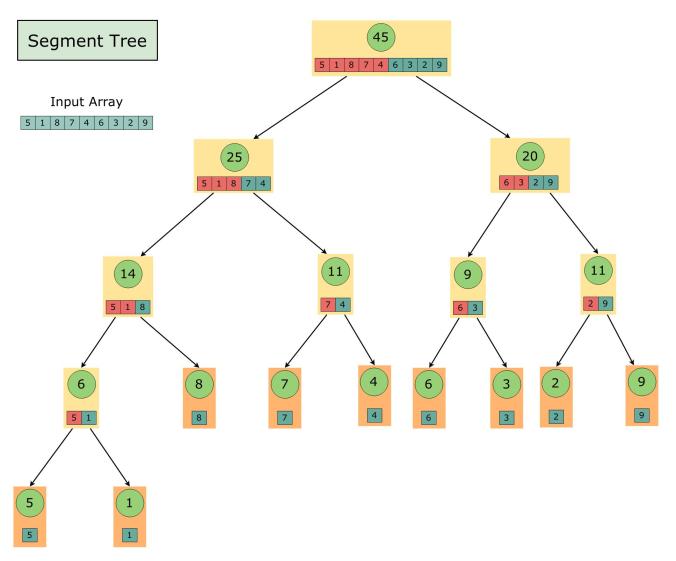
As I mentioned earlier, the Segment Tree works on the principle of partial sums. What this principle is that we somewhere hold the sum of a few elements and keep building on it. In a Segment Tree, this “partial” is actually “half”. The Segment Tree structurally is a Binary Tree. Every internal node is associated with a range of numbers, whose sum is stored in that node. Now, what we do is partition the array into two halves. The left child will hold the sum of elements in the left partition and the right child will hold the sum of elements in the right partition. You may not get the idea of Segment Tree in the first reading. That’s okay. Give another reading and ponder upon the sketch below for a better understanding.

segment1

I hope it is clear from the picture how the Segment Tree works on the partial sums, which here is the left partition sum and the right partition sum. The leaf nodes represent the individual elements of the input array.

Note that the array we will not store the array in the nodes of our Segment Tree as was depicted in the sketch. This was done in the sketch only to give you the idea. The array will not be stored in the nodes. However, we will store the range limits on which the sum is defined, i.e, we will store the start index and the end index of the span of elements in the input array whose sum is there in the node. We will use a struct for the node which looks like this –

struct node
{
	int value, low, high;
	struct node * leftChild;
	struct node * rightChild;
};

The variable ‘value’ was to store the sum, ‘low’ and ‘high’ is to store the range. The variables ‘leftChild’ and the ‘rightChild’ are to point to the children.

Building the Segment Tree –

The Segment Tree is built in a recursive manner. We could write it in a step-by-step procedure –

  • Allocate memory.
  • Start with the root.
  • Partition the array you are given into two halves.
  • Create nodes for each half.
  • The value of the parent node is the sum of values on its children.
  • This is calculated by recursively calling the procedure on the children.
  • When the array given reduces to one element. The procedure must create a node and return the value.
  • When the parent node has acquired the sum of its children, it must return its current value to carry on the recursion.

The step-by-step procedure may not be clear in the first reading. You will know what I was talking about when you understand the pseudo-code below –

int buildSegmentTree(Array, low, high, SegmentTree)
	if low == high
		SegmentTree->value = Array[low]
		SegmentTree->low = SegmentTree->high = low

		return SegmentTree->value

	mid = (low + high) / 2

	SegmentTree->low = low
	SegmentTree->high = high
	SegmentTree->leftChild = allocate memory using calloc()
	SegmentTree->rightChild = allocate memory using calloc()
	SegmentTree->value = buildSegmentTree(Array, low, mid, SegmentTree)
					   + buildSegmentTree(Array, mid + 1, high, SegmentTree)

struct node * getSegmentTree(Array, ArraySize)
	if ArraySize <= 0
		return NULL

	struct node * SegmentTree = allocate memory using calloc()

	buildSegmentTree(Array, 1, ArraySize, SegmentTree)

	return SegmentTree

I made the pseudo-code a little extra-descriptive so that you can understand the step-by-step procedure and the code simultaneously. If you have any doubts, feel free to comment them.

The time complexity of the code is O(n). This is because in the worst case we would end up building a complete binary tree which will have 2 ✗ n – 1 nodes, and we preform calculations that take O(1) time for every node.

Sum Query –

Now, it is time to discuss the two important queries that we started our discussion with. We will begin with the sum query. We are supposed to tell the sum of all the elements in a given range. Now we will use our ‘low’ and ‘high’ variables in each node of the Segment Tree. The way we do this query mimics the Binary Search. We would be given a well defined range and we will keep comparing that with the range in each node of the Tree. If it fits perfectly, then we simply return the value stored in that node. If it doesn’t we have a few cases to handle. To understand the cases, consider the following notations –

  • NodeLeft – This is the left bound of the range whose sum is stored in the node. We actually named this as ‘low’ inn our struct.
  • NodeRight – This is the right bound of the range whose sum is stored in the node. We actually named this as ‘high’ inn our struct.
  • QueryLeft – This is the left bound of the range whose sum we are supposed to calculate.
  • QueryRight – This is the right bound of the range whose sum we are supposed to calculate.
  • Mid – This is the index upon which the partition occurs to assign values to the children nodes. It is essentially the mean of NodeLeft and NodeRight.
  • Value – This is the value that the current node is holding. Same as the ‘value’ variable in our struct.

Now, let’s talk about the cases we would encounter –

  1. (NodeLeft == QueryLeft && NodeRight == QueryRight) – This is the best thing that can happen. As we discussed a moment ago, we simply return the Value.
  2. (NodeLeft >= QueryLeft && NodeRight >= QueryRight) – This is the situation where among the elements that the current node holds the sum of, a few of the elements are not needed. The range that the current node has covers more than that’s needed. Now, to proceed with the recursion, we use Mid –
    • (QueryLeft <= Mid) → getSumQuery(SegmentTree->leftChild, QueryLeft, Mid) – This condition checks if the query demands the sum of elements which are in the left partition. So, we carry on the recursion with query range concerning only the left partition.
    • (QueryRight > Mid + 1) → getSumQuery(SegmentTree->leftChild, QueryLeft, Mid) – This checks if the query wants elements of the right partition. So, we carry on the recursion with query range concerning only the right partition.

    Note that both the conditions must be checked for the sum query to give accurate results. A special case arises when (QueryLeft == QueryRight), which means that we are looking for one element, which would obviously be either in the left or the right partition. In that case, we don’t have the necessity of  checking the second condition if the first condition is already met. This is because if we know the query asks for an element in the left partition, we have nothing to do with the right partition in this case.

This will be more clear once you put this idea to work by pen-and-paper. Coding this is simple too. Once you are able to code it, you will realise its resemblance to Binary Search. In the worst case, we would have to travel all the way down the tree, which takes O(log n).

Update Query –

What do we do if we were to update an element initially given in the input. How would we have to modify our Segment Tree so that it is still correct? We know that the initial input elements can be found at the leaves of the Segment Tree. So, we should be updating that. How do we traverse down to that leaf? We do this similarly as we did it in Sum Query, where we took a range and went down the tree based on it. If we put it in Sum Query terms, QueryLeft is equal to QueryRight. We search for it in a similar fashion. Then, we update the node which we came searching for. We also keep a note of the difference, and we add the difference to all those nodes which we came by. This is because, when you update a leaf of the Segment Tree, the internal nodes which would get affected are those which contain the partial sum in which the leaf is involved. We already met those nodes in our recursive traversal. When we are “coming out” of recursion, we update them by the difference that was caused by the new value. So, basically we go down the tree and come back. So, this operation takes O(2 log n) which is O(log n).

Take a break for a while and come back to start coding the Segment Tree. You will need to do a lot of pen-and-paper work while coding this data structure. And it is totally worth it. To print your Segment Tree, you could use the Tree Walks, In-order or Pre-order or whichever pleases you. If you are getting stuck, you can always refer to my code below –

/*
 * Segment Tree
 * Data Structure
 *
 * Authored by,
 * Vamsi Sangam
 */

#include <stdio.h>
#include <stdlib.h>

struct node
{
	int value, low, high;
	struct node * leftChild;
	struct node * rightChild;
};

// The recursive procedure which actually constructs the Segment Tre
int buildSegmentTree(int arr[], int low, int high, struct node * SegmentTree)
{
	if (low == high) {
		// we have only 1 element of the array
		SegmentTree->value = arr[low];
		SegmentTree->low = SegmentTree->high = low;

		return SegmentTree->value;
	}

	// Partition
	int mid = (low + high) / 2;

	SegmentTree->low = low;			// Setting bounds to the partial sum
	SegmentTree->high = high;		// that this node is associated with

	// Creating children
	SegmentTree->leftChild = (struct node *) calloc(1, sizeof(struct node));
	SegmentTree->rightChild = (struct node *) calloc(1, sizeof(struct node));
	SegmentTree->value = buildSegmentTree(arr, low, mid, SegmentTree->leftChild)
						+ buildSegmentTree(arr, mid + 1, high, SegmentTree->rightChild);

	// Must return the value to carry on recursion
	return SegmentTree->value;
}

// Allocates memory for the root and calls method
// to construct the Segment Tree
struct node * getSegmentTree(int arr[], int n)
{
	if (n <= 0) {
		return NULL;
	}

	struct node * SegmentTree = (struct node *) calloc(1, sizeof(struct node));

	buildSegmentTree(arr, 1, n, SegmentTree);

	return SegmentTree;
}

// A utility function used for Inorder Walk
void print(struct node * SegmentTree)
{
	printf("%d -> [%d, %d]\n", SegmentTree->value, SegmentTree->low, SegmentTree->high);
}

// In-Order Walk of Segment Tree
void inOrderWalk(struct node * SegmentTree)
{
	if (SegmentTree == NULL) {
		return;
	}

	inOrderWalk(SegmentTree->leftChild);
	print(SegmentTree);
	inOrderWalk(SegmentTree->rightChild);
}

// Recursive procedure to find out the sum of elements
// from arr[low] to arr[high] using the Segment Tree
int getSumQuery(struct node * SegmentTree, int low, int high, int sum)
{
	if (low == SegmentTree->low && high == SegmentTree->high) {
		sum += SegmentTree->value;

		return sum;
	}

	if (low == high) {
		int mid = (SegmentTree->low + SegmentTree->high) / 2;

		if (low <= mid) {
			sum = getSumQuery(SegmentTree->leftChild, low, low, sum);
		} else {
			sum = getSumQuery(SegmentTree->rightChild, high, high, sum);
		}
	} else {
		int mid = (SegmentTree->low + SegmentTree->high) / 2;

		if (low <= mid) {
			sum = getSumQuery(SegmentTree->leftChild, low, mid, sum);
		}

		if (high >= mid + 1) {
			sum = getSumQuery(SegmentTree->rightChild, mid + 1, high, sum);
		}
	}

	return sum;
}

// Updates an element in the Segment Tree and makes the neccessary adjustments
int updateQuery(struct node * SegmentTree, int index, int newValue, int difference)
{
	if (SegmentTree->low == SegmentTree->high) {
		difference += newValue - SegmentTree->value;
		SegmentTree->value = newValue;

		return difference;
	}

	int mid = (SegmentTree->low + SegmentTree->high) / 2;

	if (index <= mid) {
		difference = updateQuery(SegmentTree->leftChild, index, newValue, difference);
	} else {
		difference = updateQuery(SegmentTree->rightChild, index, newValue, difference);
	}

	SegmentTree->value += difference;

	return difference;
}

int main()
{
	int n;

	printf("Enter the size of input -\n");
	scanf("%d", &n);

	int arr[n + 1], i;

	printf("\nEnter %d Integers -\n", n);

	arr[0] = -1;
	for (i = 1; i <= n; ++i) {
		scanf("%d", &arr[i]);
	}

	struct node * SegmentTree = getSegmentTree(arr, n);

	// Printing the Tree after constructing
	printf("\nIn-Order Walk of the Segment Tree -\n");
	inOrderWalk(SegmentTree);

	int low, high;

	// Demonstrating Sum Query
	printf("\nEnter the range for sum query - [1, %d]\n", n);
	scanf("%d%d", &low, &high);
	printf("\nSum = %d\n", getSumQuery(SegmentTree, low, high, 0));

	// Demonstrating Update Query
	printf("\nEnter the index of number and new value to update -\n");
	scanf("%d%d", &i, &low);
	updateQuery(SegmentTree, i, low, 0);

	// Printing the Tree after Updating
	printf("\nIn-Order Walk of the Segment Tree after Update -\n");
	inOrderWalk(SegmentTree);

	return 0;
}

There are many varieties of questions that can be asked based on this Data Structure. I’m sure you’ll start liking and appreciating this data structure as you keep solving many questions on it. If you have any doubts, feel free to comment them. I hope my post has helped you in understanding the Segment Tree. If it did, let me know by commenting…! Keep practising… Happy Coding…! 🙂
You may also like –

More in the Navigation Page ! →

Trie Tree Implementation


Hello people…! In this post we will implement an amazing data structure, the Trie Tree. Trie Trees are are used to search for all occurrences of a word in a given text very quickly. To be precise, if the length of the word is “L“, the trie tree searches for all occurrences of this data structure in O(L) time, which is very very fast in comparison to many pattern matching algorithms.

But I must mention, this data structure is not exactly used for “pattern matching”, it is used to search for the occurrences of the word in the given text. How these both functionalities differ…? We’ll get to know that shortly. The Trie Tree has many applications. Your browser could be using a trie tree internally to search for words when you press Ctrl + F. So, let’s get started with this data structure…!

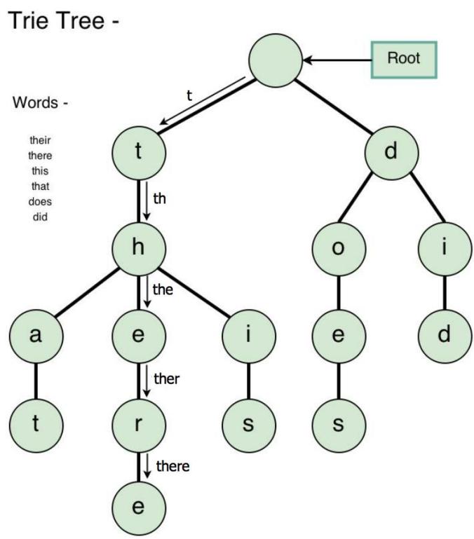
The Trie Tree is a very straight forward data structure. It is a simple tree where the nodes have an alphabet associated with them. And the way these nodes are arranged is the best part of the Trie Tree. To get an idea take a close look at the sketch below –

Structure of Trie Tree

Structure of Trie Tree

The arrows in the sketch above indicate how to traverse the trie tree in order to tell if a word exists or not. We travel through the root node, down the tree until we hit a leaf. Picking up a character at every edge, we construct our word. Now, you can easily tell why the time to search for a node in the text will be in the order of length of the word to be searched. It’s obvious…! One would have to go down till the leaf. In the worst case, one would have to travel the height of the tree which would be the length of the longest word in the whole text..! 😉

So, as we got a little idea about working with a Trie Tree, let us move on to the serious part. Let us talk about how this is implemented and then we will talk about three fundamental operations done on the Trie Tree –

  • Insert
  • Delete
  • Search

In C, the Trie Tree is implemented using structures. But the C implementation of this data structure gets a little dirty. So we will switch to C++ but we will keep it as C-ish as possible. As we keep discussing about the implementation, you will notice how many advantages we have when we use C++. This will be our structure of each node in the tree –

struct node
{
	struct node * parent;
	struct node * children[ALPHABETS];
	vector<int> occurrences;
};
  • parent – This points to the node which is the parent of the current node in the tree hierarchy. It may seem useless at the first, but we need this to travel up the tree when we want to delete any word. We’ll get to the deletion operation in a moment.
  • children – It points to the children nodes. It is made an array so that we can have O(1) accessing time. But why is the size 26…? Its simple. Consider a word, “th”, now, what could the third letter possibly be, if it had one…? One among the 26 english alphabets…! So that’s why the size is made 26. If you want to make a trie tree for another language, replace the number 26 with the number of letters in your language.
  • occurrences – This will store the starting indices of the word occurring in the given text. Now, why this is made a vector is that, vector is as good as a Linked List with random access. It is one of the most handy ready made data structures available in the C++ STL Library. If you are not familiar with vectors this is a good place to start.
    If this were C, we would have to give a fixed array size, and we would have a problem if the occurrences of a particular node are more. We could avoid this by putting a Linked List there. But we sacrifice random access and a whole lot of operations get time taking. Moreover, the code will get really really cumbersome to manage if you have a tree and a linked list.

Having got a picture of the implementation, let us look at how the operations are done in a Trie Tree.

Insert Operation

When we do an insert operation, there are a few cases –

  1. The word to be inserted does not exist.
  2. The word to be inserted already exists in the tree.
  3. The word to be inserted does not exists, but as the suffix of a word.

The first case is simple. One would have to traverse till the alphabets of the words have nodes in the trie tree or else create new nodes one-after-the-other. And at the end of the word, i.e., the node for the last alphabet, we will mark it as a leaf and push the starting index into the vector indicating the occurrence of the newly inserted word.

During this course of traversal, we will be cutting off the string of the word we have one-by-one as they are processed. This is done by putting using a vector of characters and popping off one character after the other. This is less code to handle and more efficient as we can use a vector as a queue. This is another advantage of using C++.

After having learnt what to do with the first case, you can guess what we would have to do in the second case. We simply have to add a new value to the occurrences vector at the node corresponding to the last alphabet of the word. We can also know the number of occurrences in constant time, we simply return the size of the vector. This is another advantage of using C++.

To understand the challenge in the third case, let’s take a simple example. What would you do with your trie tree if you wanted to insert the word “face” if the word “facebook” is already there in your tree…? This is the third case. The answer to this is the occurrence vector itself. We simply push the starting index of the word into the vector of that node which corresponds to the last alphabet of the word to be inserted, in the above example, this would be the node of “e”. So, what really tells if there’s a word ending with the alphabet corresponding to the current node is the size of the vector.

So I hope you understand how important our vector is. A lot depends on it…!

Delete Operation

The deletion of a word in the trie tree is similar to the insertion, we have a few cases –

  • Error 404 : Word not found…!
  • Word exists as a stand-alone word.
  • Word exists as a prefix of another word.

If the word is not there at all, we don’t have to do anything. We just have to make sure that we don’t mess up the existing data structure…!

The second case is a little tricky. We would have to delete the word bottom-up. That is, we will delete that part of the word which is not a part of any other word. For example, consider the sketch above. If we were to delete “this”, we would delete the letters ‘i’ and ‘s’ as, ‘h’ is a part of another word. This keeps us away from distorting the data structure. If the word were existing multiple number of times we will simply remove the occurrence from the vector of the concerned node.

In the third case too, we will simply delete the occurrence of the word from the vector. We needn’t write a lot of code as we can use the functions in algorithm header file. This is another advantage of using C++.

Note – When we delete the occurrence of a word, we are not concerned about the validity of the indices stored as occurrences of other words. What I mean to say is, suppose we have 10 words. If we delete the 3rd word, the 5th word or the 9th word is supposed to become the 4rth and the 8th word as far as the original text is concerned. But we will not consider this. The data stored in the trie tree is not meant to me deleted or inserted. The Trie Tree is meant for processing the given text not to manipulate the given text.

Search Operation

The search operation is simple and is as we discussed when we began our discussion about the Trie Tree. We go down the tree traversing the nodes and keep “picking up characters” as we go. And the occurrences vector tells us if a word exists that ends with the alphabet associated with the current node, and if so, it gives us the indices of occurrences and also the number of occurrences.

Besides these basic operations, there is another very interesting operation that is done with the Trie Tree –

  • Lexicographical Sort – If we want to print all the words processed into the trie tree lexicographically, all we have to do is do a Preorder Walk on the tree. This will automatically print all the words in the lexicographical order or the dictionary order. This is due to the very structure and arrangement of nodes in a Trie Tree. Now, I’d like to share another interesting thing about pre-order walk in trees… The Pre-order walk works exactly as a Depth First Search (DFS) in graphs, i.e., the sequence in which both the algorithms visit the nodes is the same. Think about this for a while and word out the two algorithms on an example (you could take mine in the sketch above), and you can see why it is so. You will also notice why the printed words would be lexicographically sorted.

Now, having learned a lot about the trie tree, try coding it in C++. If you are uneasy with C++, you can try it in C, but make sure you try at least 3 times. Trying is very important. I don’t know if you are new to reading my posts, but I insist a lot on trying in every post of mine…! If you have succeeded, you’re fabulous…! If not, check out my code below any try figuring out how just close you were…!!

/* ==========  ========== ========== ========= */
//          Trie Tree Data Structure           //
//                using C++ STL                //
//                                             //
//         Functions follow Pascal Case        //
//           Convention and Variables      	   //
//         follow Camel Case Convention        //
//                                             //
//            Author - Vamsi Sangam            //
//            Theory of Programming            //
/* ========== ========== ========== ========== */

#include <cstdio>
#include <cstdlib>
#include <vector>

#define ALPHABETS 26
#define CASE 'a'
#define MAX_WORD_SIZE 25

using namespace std;

struct Node
{
    struct Node * parent;
    struct Node * children[ALPHABETS];
    vector<int> occurrences;
};

// Inserts a word 'text' into the Trie Tree
// 'trieTree' and marks it's occurence as 'index'.
void InsertWord(struct Node * trieTree, char * word, int index)
{
    struct Node * traverse = trieTree;

    while (*word != '\0') {     // Until there is something to process
        if (traverse->children[*word - CASE] == NULL) {
            // There is no node in 'trieTree' corresponding to this alphabet

            // Allocate using calloc(), so that components are initialised
            traverse->children[*word - CASE] = (struct Node *) calloc(1, sizeof(struct Node));
            traverse->children[*word - CASE]->parent = traverse;  // Assigning parent
        }

        traverse = traverse->children[*word - CASE];
        ++word; // The next alphabet
    }

    traverse->occurrences.push_back(index);      // Mark the occurence of the word
}

// Searches for the occurence of a word in 'trieTree',
// if not found, returns NULL,
// if found, returns poniter pointing to the
// last node of the word in the 'trieTree'
// Complexity -> O(length_of_word_to_be_searched)
struct Node * SearchWord(struct Node * treeNode, char * word)
{
    // Function is very similar to insert() function
    while (*word != '\0') {
        if (treeNode->children[*word - CASE] != NULL) {
            treeNode = treeNode->children[*word - CASE];
            ++word;
        } else {
            break;
        }
    }

    if (*word == '\0' && treeNode->occurrences.size() != 0) {
        // Word found
        return treeNode;
    } else {
        // Word not found
        return NULL;
    }
}

// Searches the word first, if not found, does nothing
// if found, deletes the nodes corresponding to the word
void RemoveWord(struct Node * trieTree, char * word)
{
    struct Node * trieNode = SearchWord(trieTree, word);

    if (trieNode == NULL) {
        // Word not found
        return;
    }

    trieNode->occurrences.pop_back();    // Deleting the occurence

    // 'noChild' indicates if the node is a leaf node
    bool noChild = true;

    int childCount = 0;
    // 'childCount' has the number of children the current node
    // has which actually tells us if the node is associated with
    // another word .This will happen if 'childCount' != 0.
    int i;

    // Checking children of current node
    for (i = 0; i < ALPHABETS; ++i) {
        if (trieNode->children[i] != NULL) {
            noChild = false;
            ++childCount;
        }
    }

    if (!noChild) {
        // The node has children, which means that the word whose
        // occurrence was just removed is a Suffix-Word
        // So, logically no more nodes have to be deleted
        return;
    }

    struct Node * parentNode;     // variable to assist in traversal

    while (trieNode->occurrences.size() == 0 && trieNode->parent != NULL && childCount == 0) {
        // trieNode->occurrences.size() -> tells if the node is associated with another word
        //
        // trieNode->parent != NULL -> is the base case sort-of condition, we simply ran
        // out of nodes to be deleted, as we reached the root
        //
        // childCount -> does the same thing as explained in the beginning, to every node
        // we reach

        parentNode = trieNode->parent;

        for (i = 0; i < ALPHABETS; ++i) {
        	if (parentNode->children[i] != NULL) {
        		++childCount;

        		if (trieNode == parentNode->children[i]) {
	                parentNode->children[i] = NULL;
	                free(trieNode);
	        		trieNode = parentNode;
	            }
			}
        }
    }
}

// Prints the 'trieTree' in a Pre-Order or a DFS manner
// which automatically results in a Lexicographical Order
void LexicographicalPrint(struct Node * trieTree, vector<char> word)
{
    int i;
    bool noChild = true;

    if (trieTree->occurrences.size() != 0) {
        // Condition trie_tree->occurrences.size() != 0,
        // is a neccessary and sufficient condition to
        // tell if a node is associated with a word or not

        vector<char>::iterator charItr = word.begin();

        while (charItr != word.end()) {
            printf("%c", *charItr);
            ++charItr;
        }
        printf(" -> @ index -> ");

        vector<int>::iterator counter = trieTree->occurrences.begin();
        // This is to print the occurences of the word

        while (counter != trieTree->occurrences.end()) {
            printf("%d, ", *counter);
            ++counter;
        }

        printf("\n");
    }

    for (i = 0; i < ALPHABETS; ++i) {
        if (trieTree->children[i] != NULL) {
            noChild = false;
            word.push_back(CASE + i);   // Select a child

            // and explore everything associated with the cild
            LexicographicalPrint(trieTree->children[i], word);
            word.pop_back();
            // Remove the alphabet as we dealt
            // everything associated with it
        }
    }

    word.pop_back();
}

int main()
{
    int n, i;
	vector<char> printUtil;		// Utility variable to print tree

	// Creating the Trie Tree using calloc
	// so that the components are initialised
    struct Node * trieTree = (struct Node *) calloc(1, sizeof(struct Node));
    char word[MAX_WORD_SIZE];

	printf("Enter the number of words-\n");
    scanf("%d", &n);

    for (i = 1; i <= n; ++i) {
        scanf("%s", word);
        InsertWord(trieTree, word, i);
    }

    printf("\n");   // Just to make the output more readable
    LexicographicalPrint(trieTree, printUtil);

    printf("\nEnter the Word to be removed - ");
    scanf("%s", word);
    RemoveWord(trieTree, word);

    printf("\n");   // Just to make the output more readable
    LexicographicalPrint(trieTree, printUtil);

    return 0;
}

The code is highly commented with explanation. It is well described, but if you have any doubts regarding the data structure or the code, feel free to comment them. I have used a few macros. The macro CASE indicates for which case the Trie Tree works. If we mention ‘A’ as the macro, the Trie Tree will work for upper case words only.

Other Implementations

The code is well tested against fairly large input. You can download the test case file here – Trie Tree Input (PDF). You can just clock your code for the insert operations. My code took 1.236 seconds to execute that loop which reads a word and inserts it into the Trie Tree. There are 5000 words in total. The last word in the input file is the word to be deleted.

If you think you can give a suggestion to make my code better, please do comment them too. I appreciate your suggestions. For those there who are struggling to get their code right, “Keep the effort going guys”…! Remember, you won’t learn anything if you keep writing Hello World program again and again. So, keep practicing…! I hope my post has helped you in getting to know about the Trie Tree. If it did, let me know by commenting ! Happy Coding…! 😀

Binary Indexed Tree (or) Fenwick Tree


Every programmer needs a suitable data structure to compute some complex function or to do a time-taking task quickly. In this post, I will explain the Binary Indexed Tree (BIT) data structure also known as the Fenwick Tree in post-soviet countries. This data structure is very easy to code in competitions. So, a programmer who knows BIT will have a massive edge over others. But the problem with BIT is that it is NOT easy to understand! A beginner may go nuts in trying to understand the working of a Binary Indexed Tree. I will explain this data structure step-by-step using as many images, tables and examples as I can.

Binary Indexed Tree becomes handy in manipulating Cumulative Frequency Tables. Now, I assume you know what Frequency and Cumulative Frequency is! Now, consider we have 12 objects with us of the respective frequencies –

Item No. Frequency Cumulative Frequency
1 4 4
2 2 6
3 7 13
4 5 18
5 1 19
6 3 22
7 6 28
8 4 32
9 6 38
10 6 44
11 3 47
12 3 50

Now, if we were to increase the quantity of Item 5 by 1. We would have to change the whole table. The change would be like,

Item No. Frequency Cumulative Frequency
1 4 4
2 2 6
3 7 13
4 5 18
5 1 + 1 19 + 1
6 3 22 + 1
7 6 28 + 1
8 4 32 + 1
9 6 38 + 1
10 6 44 + 1
11 3 47 + 1
12 3 50 + 1

If we were to code this manipulation using an array of integers, the implementation would go like,

Array Element Element Value
arr[0] 4
arr[1] 6
arr[2] 13
arr[3] 18
arr[4] 19 + 1
arr[5] 22 + 1
arr[6] 28 + 1
arr[7] 32 + 1
arr[8] 38 + 1
arr[9] 44 + 1
arr[10] 47 + 1
arr[11] 50 + 1

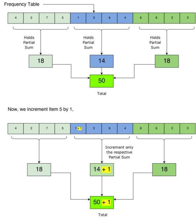
Clearly, implementing the simple increment would cost O(n). This is because in Cumulative Frequency, every element holds the “prefix-sum” of the elements, i.e., the sum of elements till that index. Now what if we hold only partial sums? Say, there are three variables that hold the partial sums and the final sums can be evaluated by summing up the partial sum. Now, the question arises is, “How does this help the increment manipulation?”. This is explained by the following diagram.

bit1

So, we can see how by using the Partial Sum Technique, we managed to decrease the number of operations to perform. This is the raw underlying idea of the Binary Indexed Tree. But the Binary Indexed Tree uses this partial sum technique far more efficiently and quite amazingly actually! The BIT is constructed on the principle that “all numbers can be represented as the sums of powers of 2”. This is more or less similar to the principle behind the binary numbers. Now the working of the BIT is that, at indices
of the values of powers of 2, they contain the total sum of the frequencies till that index. Which means if we have an element of an array, arr[7], it will have the sum of elements from arr[0] to arr[7] (including the value of arr[7], i.e, frequency of the 8th element). Thats ok! But what will the other elements contain…?! The Partial Sums…! I make this clear with the help of my next sketch where I show a simple Binary Search Tree (BST) where the nodes have the values of the frequencies and the nodes are constructed in such a way that the value of the “index” is taken into consideration while constructing the BST but the nodes hold the frequencies as the values. Then I will give a super simple step-by-step explanation.

bit2

We all know that the Binary Search Tree is such that the left-subtree holds all the values less than the current node. Now, the Binary Indexed tree is such that, the current node holds the sum of all values in it’s left-subtree + the value of the current node. For example, in the first tree in the above image,

Value of Node 10 = Value of Node 9 + Value of Node 10

Value of Node 12 = Values of Node 12 + Value of Node 10 (= Value of Node 9 + Value of Node 10…!)

Similarly,

Value of Node 4 = Values of Node 4 + Value of Node 3 + Value of Node 2 (= Value of Node 2 + Value of Node 1…!)

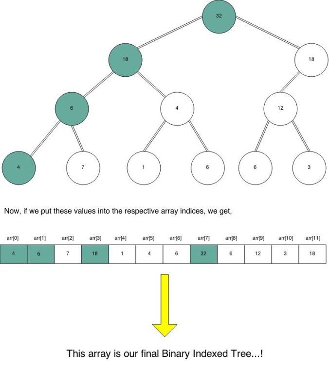
So, now we see that the Node 4 will be the sum of Nodes 1 to 4, similar is the case with all the nodes that are powers of 2. These nodes are somewhat special, as they contain the “prefix-sum”. Hence, I marked them in my previous image. Now we will apply the concept to our second tree in the above image.

bit3

Wait…! What…?! The “array” is the “tree”…?! Yes…! The array we obtained is called the Binary Indexed Tree. For whatever applications a BIT is used for, it is used as this array. Pretty cool, uh…! So, this means you don’t have to get messed up creating structures, pointers and doing tree travels! All you’ll need is this simple array. Now, before we get into the coding part of the BIT lets observe this BIT “array” a little more closely so that we can understand it more clearly. Again, I use an image because we all know, “A picture speaks more than a thousand words!”.

bit4

The picture clearly shows how the Fenwick Tree (or BIT) stores the partial sums and that at indices of powers of two it will have the complete sum of all the elements behind it. What really allows the Fenwick Tree to have this feature is the very structure of the Binary Search Tree (BST). In a BST, the nodes with index in powers of two lie at the left-most part of the tree (recall our very first tree of the first image), now, we know for a Binary Indexed Tree, the value of a node is the sum of the components of the left-subtree + the value that is supposed to be in that node. But what will the left-subtree of a Binary Search Tree have?… “Some” elements surely less than it. Now, what will the left-subtree of the left-most wing of a tree have? “All” the elements surely less than it. If you ponder on this statement for a while you will understand why the indices of the powers of 2 have the whole “prefix-sum”. Now I will depict you the effect of increment of an Item in the Binary Indexed Tree, for this I use the tree representation once again.

bit5-2

As we can clearly see, in a worst case scenario, such as the above, we’d have to update all the nodes beginning from the lowest level and go up till the root node. So, in a worst case scenario, we’d have to update the “height of the tree” number of nodes, which is log n as we know it. So, the increment operation here costs only O(log n), which is very fast! Recall that our brute force or the naive approach costed us O(n), so now we know how using BIT speeds up the manipulation. But how do we do this in an array? For a given frequency table, how do we construct the BIT? We will see this coding part now, which is also difficult to understand but easy to implement.

For a given frequency array freq[] of size ‘n’, create another array bit[] of size ‘n’ and initialize bit[] to zero. Now, run a loop where we take every element of freq[] one-by-one and put it into bit[]. What actually are we doing is that we are doing the increment operation over and over again. Look over the code closely –

/*
 * Code to generate Fenwick Tree
 * from a given Frequency Table
 *
 * by,
 * Vamsi Sangam
 */

#include <stdio.h>

int main()
{
	int n, i, j;

	printf("Enter size of Frequency Table = ");
	scanf("%d", &n);

	int freq[n + 1];

	printf("Enter numbers to Frequency Table -\n");

	for (i = 1; i <= n; ++i) {
		scanf("%d", &freq[i]);
	}

	printf("\n");

	int bit[n + 1];

	for (i = 1; i <= n; ++i) {
		bit[i] = 0;
	}

	printf("Initial Fenwick Tree -\n");
	for (i = 1; i <= n; ++i) {
		printf("%d      ", bit[i]);
	}

	printf("\n\nThe Fenwick Tree stages per iterate -\n");

	for (i = 1; i <= n; ++i) {
		j = i;
		printf("freq[%d] = %d\n", i, freq[i]);
		while (j <= n) {
			bit[j] += freq[i];
			j = j + (j & (-j));
		}

		for (j = 1; j <= n; ++j) {
			printf("%d      ", bit[j]);
		}
		printf("\n\n");
	}

	printf("\nThe Final Fenwick Tree is - \n");
	for (i = 1; i <= n; ++i) {
		printf("%d ", bit[i]);
	}

	return 0;
}

You might feel uncomfortable with the “j = j + (j & (-j))” thing, for now, forget that, we’ll come back to it in a minute. Look what is logically happening in the code. Being able to read raw code is a gift, if you can, you’re awesome! Be proud of it! For those who can’t, here is what happening. Listen carefully!… First we take the collection of items to be empty, so, all items have zero frequency. Then, we take the first item, it’s frequency is 4, so we “increment” the frequency of that item from 0 → 4. Now, recall the picture of the effect of increment in Fenwick Trees. I drew a Binary Search Tree and incremented the leaf node and up till the root by 1. Here, we will increment by 4, all the corresponding log n nodes. For better understanding watch the picture below closely –

bit6

It is clear from the explanation how the Fenwick Tree gets going. But how does one traverse so strangely, I mean, the first Item we had to go like, 1 → 2 → 4 → 8, then for the next Item we had to go like, 2 → 4 → 8, and then like 3 → 4 → 8…! How does one put it in a code? This is exactly what “j = j + (j & (-j))” does! It takes you to the next location where you are to increment the value. It is a standard expression for traversing a Fenwick Tree. If you are really eager to understand the logic behind the standard expression, you have to read this wonderful blog by Devendra Agarwal. It was where I was able to start my BIT journey. Lastly, I will just show you an output of the same above code but with little modification so that it prints the values of variables and BIT array step-by-step.

If you have understood till here, you will be able to understand the output without breaking a sweat. I will conclude this post here. It has become too large already, and I guess my reader’s would also like a break. Thanks a lot for being so patient with me! If you really are eager to do some questions on this topic, go for Insertion Sort Advanced Analysis of HackerRank. I enjoyed solving that question, and I hope you will too! Feel free to comment your doubts..! Commenting is super easy if you are a Facebook, Twitter or a Google+ user…! So, don’t hesitate..! 😉 … Keep practising…! Happy Coding…! 🙂

Famous 5 in Theory of Programming !

More in the Navigation Page ! →