Prim’s Algorithm


Hello people…! In this post, I will talk about the Prim’s Algorithm for finding a Minimum Spanning Tree for a given weighted graph. It is an excellent example of a Greedy Algorithm. It is very similar to Dijkstra’s Algorithm for finding the shortest path from a given source. This is my first post regarding the minimum spanning tree, so, let’s take some time to learn what a minimum spanning tree is.

Minimum Spanning Tree – A spanning tree is a connected and acyclic graph. It has |V| – 1 edges. For a given graph, we could have many spanning trees. A minimum spanning tree is the one which has the minimum sum of all edges when compared to all the possible spanning trees that can be formed from the given graph.

Why would anyone bother about a minimum spanning tree..? Minimum spanning trees are used in certain places to get the job done faster. It is used in a network router to find the routes to other components in the network such that the transfer of a data packet would consume the least amount of resources. Minimum spanning trees are used in a whole lot of other aspects of computer science. So, let’s get started !

If you already know Dijkstra’s Algorithm, you could relate to the similarities between these two algorithms. But, let’s assume that you don’t know Dijkstra’s Algorithm, and begin Prim’s Algorithm from scratch. Before we get started with the algorithm, let’s look at the tools we would be needing –

  • Priority Queue – We will be using a Binary Min-Heap with an array-based implementation with a small twist. The array here will be an STL vector. This is because, during the course of our algorithm, this priority queue will grow and shrink.
  • Visited array – We will be using a Boolean array of size |V| to keep a check on which nodes have been visited and which haven’t been visited.
  • Extra Adjacency List – Beside the input Adjacency List, we will have another empty Adjacency List where we will keep filling it with vertices. This will become our final minimum spanning tree.

Beside these, we will use other variables to aid our algorithm, but these are our main tools. Now, let’s look at a crude step-by-step version of the Prim’s Algorithm –

  • Start from any arbitrary vertex.
  • Note down all the edges emerging from this vertex.
  • Mark this edge as visited.
  • Select an edge with the minimum weight.
  • Traverse to the other end. Remove this edge from the list and insert it into the minimum spanning tree.
  • Repeat this process for the newly visited vertex.
  • Each time you visit a vertex, check if it was already visited, only then we do the process of adding its edges to the list and picking the minimum.
  • If not, then simply pick up the next minimum edge.
  • Repeat this process until all the nodes are visited.

This is the raw idea of the Prim’s Algorithm. Now, I hope you can figure out the why we would need the tools I stated above. The list into which we are adding edges is our priority queue. We will be adding and removing edges into it as we move forward in the algorithm. We will be adding the edges into the minimum spanning tree, so we need the extra adjacency list. To check whether a vertex has been visited or not, we will need the Boolean array.

But there’s another thing of interest from the coding point of view. It is stated that if we come to a vertex that we have already visited, we extract the next minimum from our list (priority queue). But, this edge could be connecting two vertices which the current vertex may not be a part of. Think about this for a while ! It is not enough if we simply keep inserting edge weights into the list. We must be precisely be able to recognize an edge from the rest. Therefore, we must store all the attributes that an edge has. Which are –

  • Start vertex.
  • End vertex.
  • Weight.

So, this tells something about our priority queue. Each element in the priority queue must be a struct of these three integers. So, our priority queue would be a vector of structures, where the structure looks like this –

struct edge
{
	int u;
	int v;
	int weight;
};

It denotes that there is an edge u → v, with a weight of ‘weight’. Now, keep reading the step-by-step process till you are comfortable with the idea. And now, let’s refine our idea of Prim’s Algorithm by writing the pseudo-code –

prims(adjacencyList, vertices, startVertex, MST)
	current = startVertex

	for i = 0 to vertices
		visited[i] = false

	i = 0

	while i < vertices
		if !visited[current]
			visited[current] = true
			temp = adjacencyList[current]

			while temp != NULL
				var.u = current
				var.v = temp->val
				var.weight = temp->weight
				PriorityQueue.enqueue(var)
				temp = temp->next

			var = PriorityQueue.extractMin();
			newVertex = var.v
			current = var.u

			if !visited[newVertex]
				MST[current] = addEdge(MST[current], newVertex, var.weight)
				MST[newVertex] = addEdge(MST[newVertex], current, var.weight)

			current = newVertex
			++i
		else
			var = PriorityQueue.extractMin();
			newVertex = var.v
			current = var.u

			if !visited[newVertex]
				MST[current] = addEdge(MST[current], newVertex, var.weight)
				MST[newVertex] = addEdge(MST[newVertex], current, var.weight)

			current = newVertex

Or, if we put the same thing in much simpler English –

prims(InputGraph, vertices, startVertex, MST)
	initialise visited array to false
	count = 0	// counts vertices visited

	while count < vertices // there are vertices to visit
		if current node not visited
			mark it visited
			push all its edges to the PriorityQueue
			extract the minimum edge from PriorityQueue

			if the minimum edge leads to an unvisited vertex
				add it to MST

			current = newVertex
			++count
		else
			extract the minimum edge from PriorityQueue again

			if the minimum edge leads to an unvisited vertex
				add it to MST

			current = newVertex

I hope the pseudo-code gives you an idea of what is to be done in Prim’s Algorithm. If not, feel free to ask your doubts..! To understand the working of the algorithm, let’s take up an sample graph and apply the above algorithm. The sketch below applies the Prim’s Algorithm on a given graph to compute the Minimum Spanning Tree –

prims1


I hope the sketch makes it clear how the Prim’s Algorithm works. Feel free to ask, if you have any doubts…!

The Priority Queue

Now, coming to the programming part of the Prim’s Algorithm, we need a priority queue. There are many ways to implement a priority queue, the best being a Fibonacci Heap. But, we will keep it simple and go for a Min – Heap. Now. As stated before, we need each node in the heap to store information about the startVertex, endVertex and the weight of the edge. So, we will use an array based implementation of the Min Heap, where the array will be an array of structures, where the priorities are based on edge weights. So, code for the priority queue goes in that fashion.

/*
 * Priority Queue (Min Heap)
 * implementation by Arrays
 * for Prim's Algorithm
 *
 * Authored by,
 * Vamsi Sangam
 */

#include <stdio.h>
#include <stdlib.h>

struct edge
{
	int u, v;
	int weight;
};

void Enqueue(struct edge heap[], int size, struct edge value)
{
	heap[size] = value;

	int i = size;
	struct edge temp;

	while (i >= 1) {
		if (heap[i / 2].weight > heap[i].weight) {
			//Parent node is greater than Child Node
			//Heap Property violated
			//So, swap
			temp = heap[i / 2];
			heap[i / 2] = heap[i];
			heap[i] = temp;

			i = i / 2;
		} else {
			//Parent is less or equal to the child
			//Heap property not violated
			//So, Insertion is done, break
			break;
		}
	}
}

void Heapify(struct edge heap[], int size, int index)
{
	int i = index;
	struct edge temp;

	while ((2 * i) < size) {
		//Left Child exists

		if ((2 * i) + 1 >= size) {
			//Right child does not exist, but left does
			if (heap[i].weight > heap[2 * i].weight) {
				//Left child is smaller than parent
				temp = heap[i];
				heap[i] = heap[2 * i];
				heap[2 * i] = temp;
				break;
				//Once you reach this level where it does not
				//have a right child, the heap ends here
				//taking it to the next iteration is pointless
			}
		}

		//Both Children exist
		if (heap[i].weight > heap[2 * i].weight || heap[i].weight > heap[2 * i + 1].weight) {
			//One of the other child is lesser than parent
			//Now find the least amoung 2 children

			if (heap[2 * i].weight <= heap[(2 * i) + 1].weight) {
				//Left Child is lesser, so, swap
				temp = heap[2 * i];
				heap[2 * i] = heap[i];
				heap[i] = temp;
				//And go down the heap
				i = 2 * i;
			} else if (heap[2 * i].weight > heap[(2 * i) + 1].weight) {
				//Left Child is lesser, so, swap
				temp = heap[(2 * i) + 1];
				heap[(2 * i) + 1] = heap[i];
				heap[i] = temp;
				//And go down the heap
				i = (2 * i) + 1;
			}
		} else {
			//Parent is lesser than its children
			break;
		}
	}
}

void DeleteNode(struct edge heap[], int size, int index)
{
	//Swap the indexed element with the last
	struct edge temp = heap[index];
	heap[index] = heap[size - 1];
	heap[size - 1] = temp;

	int i = index;
	--size;

	Heapify(heap, size, i);
}

Other implementations of Prim’s Algorithm

All I did was I took the code in my post regarding Binary Heaps, and modified it to work on an array of structures. And I added a new function ExtractMin() which returns the element with the minimum priority, essentially deleting it from the Min Heap. Go through the code of the Priority Queue until you get comfortable with it. You could add a main function to test the code and know for yourself how it works. It would be even better if you took your own (or mine) implementation of Binary Heap and modified it to support Prim’s Algorithm on your own.

The Algorithm

Once you have your Priority Queue ready, it is pretty easy to code the Prim’s Algorithm looking at the pseudo-code. But there is one coding issue. The Priority Queue here is an array, which obviously must be of fixed length. But in the algorithm, the edges are continuously added and extracted from the queue. So, what should our array size be….? If you notice, throughout the algorithm, we add every edge at most twice. So, the maximum possible size of the queue would be 2 ✗ |E|. So, you could keep the array size as this, or, you could optimize the algorithm by ensuring that an edge is not inserted twice. This will increase your efficiency in terms of memory usage and computations. But how do you do this..? While adding an edge, check if it is leading to a vertex which has already been visited. If not, only then we insert it into the Min Heap. Well, first try to code it without the optimization, if you succeed then optimizing it shouldn’t be difficult. If you get stuck, you can refer to my code below, which is the optimized version…!

/*
 * Prim's Algorithm
 * using a Min Heap
 *
 * Authored by,
 * Vamsi Sangam.
 *
 */

#include <cstdio>
#include <cstdlib>

using namespace std;

struct node {
    int val;
    int weight;
    struct node * next;
};

struct edge {
	int weight;
	int u, v;	// edge from u ---> v
};

// Adds an edge to an Adjacency List element
struct node * addEdge(struct node * head, int num, int weight)
{
    struct node * p = (struct node *) malloc(sizeof(struct node));

    p->val = num;
    p->next = head;
    p->weight = weight;
    head = p;

    return p;
}

// Enqueues an entry into the Priority Queue
void Enqueue(struct edge heap[], int size, struct edge value)
{
	heap[size] = value;

	int i = size;
	struct edge temp;

	while (i >= 1) {
		if (heap[i / 2].weight > heap[i].weight) {
			temp = heap[i / 2];
			heap[i / 2] = heap[i];
			heap[i] = temp;

			i = i / 2;
		} else {
			break;
		}
	}
}

void Heapify(struct edge heap[], int size, int index)
{
	int i = index;
	struct edge temp;

	while ((2 * i) < size) {
		if ((2 * i) + 1 >= size) {
			if (heap[i].weight > heap[2 * i].weight) {
				temp = heap[i];
				heap[i] = heap[2 * i];
				heap[2 * i] = temp;

				break;
			}
		}

		if (heap[i].weight > heap[2 * i].weight || heap[i].weight > heap[2 * i + 1].weight) {
			if (heap[2 * i].weight <= heap[(2 * i) + 1].weight) {
				temp = heap[2 * i];
				heap[2 * i] = heap[i];
				heap[i] = temp;

				i = 2 * i;
			} else if (heap[2 * i].weight > heap[(2 * i) + 1].weight) {
				temp = heap[(2 * i) + 1];
				heap[(2 * i) + 1] = heap[i];
				heap[i] = temp;

				i = (2 * i) + 1;
			}
		} else {
			break;
		}
	}
}

// Deletes and entry in the Priority Queue
void DeleteNode(struct edge heap[], int size, int index)
{
	struct edge temp = heap[index];

	heap[index] = heap[size - 1];
	heap[size - 1] = temp;

	int i = index;
	--size;

	Heapify(heap, size, i);
}

// Returns the element with
// Minimum Priority and deletes it
struct edge ExtractMin(struct edge heap[], int size)
{
	struct edge min = heap[0];

	DeleteNode(heap, size, 0);

	return min;
}

// Prim's Algorithm function
void Prim(struct node * adjacencylist[], int vertices, int edges, int startVertex, struct node * MST[])
{
	int current = startVertex, newVertex;
	bool visited[vertices + 1];
	struct node * temp;
	struct edge var;
	struct edge PriorityQueue[2 * edges];
	int QueueSize = 0;

	int i;

	for (i = 0; i <= vertices; ++i) {		// Initializing
		visited[i] = false;
	}

	i = 0;

	while (i < vertices) {
		if (!visited[current]) {			// If current node is not visited
			visited[current] = true;		// Mark it visited
			temp = adjacencylist[current];

			while (temp != NULL) {
				var.u = current;
				var.v = temp->val;
				var.weight = temp->weight;

				if (!visited[var.v]) {
					// If the edge leads to an un-visited
					// vertex only then enqueue it
					Enqueue(PriorityQueue, QueueSize, var);
					++QueueSize;
				}

				temp = temp->next;
			}

			var = ExtractMin(PriorityQueue, QueueSize);		// The greedy choice
			--QueueSize;

			newVertex = var.v;
			current = var.u;

			if (!visited[newVertex]) {
				// If it leads to an un-visited vertex, add it to MST
				MST[current] = addEdge(MST[current], newVertex, var.weight);
				MST[newVertex] = addEdge(MST[newVertex], current, var.weight);
			}

			current = newVertex;
			++i;
		} else {

			var = ExtractMin(PriorityQueue, QueueSize);
			--QueueSize;

			newVertex = var.v;
			current = var.u;

			if (!visited[newVertex]) {
				MST[current] = addEdge(MST[current], newVertex, var.weight);
				MST[newVertex] = addEdge(MST[newVertex], current, var.weight);
			}

			current = newVertex;
		}
	}
}

int main()
{
    int vertices, edges, i, j, v1, v2, weight;

    printf("Enter the Number of Vertices -\n");
    scanf("%d", &vertices);

    printf("Enter the Number of Edges -\n");
    scanf("%d", &edges);

    struct node * adjacency_list[vertices + 1];
    struct node * MST[vertices + 1];

    for (i = 0; i <= vertices; ++i) {
        adjacency_list[i] = NULL;
        MST[i] = NULL;
    }

    for (i = 1; i <= edges; ++i) {
        scanf("%d%d%d", &v1, &v2, &weight);
        adjacency_list[v1] = addEdge(adjacency_list[v1], v2, weight);       //Adding edge v1 ---W---> v2
        adjacency_list[v2] = addEdge(adjacency_list[v2], v1, weight);       //Adding edge v2 ---W---> v1
    }

    // Printing Adjacency List
    printf("\nAdjacency List -\n\n");
    for (i = 1; i <= vertices; ++i) {
        printf("adjacency_list[%d] -> ", i);

        struct node * temp = adjacency_list[i];

        while (temp != NULL) {
            printf("%d -> ", temp->val);
            temp = temp->next;
        }

        printf("NULL\n");
	}

	int startVertex;

	printf("\nEnter a Start Vertex - ");
	scanf("%d", &startVertex);
	Prim(adjacency_list, vertices, edges, startVertex, MST);

	// Printing MST
	printf("\nMinimum Spanning Tree -\n\n");
	for (i = 1; i <= vertices; ++i) {
		printf("MST[%d] -> ", i);

		struct node * temp = MST[i];

		while (temp != NULL) {
            printf("%d -> ", temp->val);
            temp = temp->next;
        }

        printf("NULL\n");
	}

    return 0;
}

If not for the Boolean array, everything else is C. So, this code shouldn’t look alien to you. This was the Prim’s Algorithm. Now, let’s talk about the complexity –

  • We perform at most |E| insert operations into the Min Heap, where each costs O(log |E|), so that makes up, O(|E| log |E|).
  • We perform at most |E| extract min operations, where each costs O(log |E|), so that makes up, O(|E| log |E|).

So, the worst case complexity of the Prim’s Algorithm is O(|E| log |E|), which is okay, but not great if the given graph is a dense graph, where |E| would be in the order of |V|2. The algorithm can be optimized further to improve the complexity to O(|E| log |V|), using a Min Heap as the Priority Queue itself. We will discuss that implementation shortly.

I hope my post has helped you in getting started with the Prim’s Algorithm. If it did, let me know by commenting…! Commenting is super easy if you are a Facebook, Twitter or a Google+ user…! So, don’t hesitate..! 😉 … Keep practising… Happy Coding…! 🙂

You may also like –

More in the Navigation Page ! →

Bellman Ford Algorithm


Hello people…! In this post I will talk about another single source shortest path algorithm, the Bellman Ford Algorithm. Unlike Dijkstra’s Algorithm, which works only for a graph positive edge weights, the Bellman Ford Algorithm will give the shortest path from a given vertex for a graph with negative edge weights also. Due to this, the Bellman Ford Algorithm is more versatile, but, it’s speciality comes at a cost. The runtime complexity of Bellman Ford Algorithm is O(|V||E|), which is substantially more than that of Dijkstra’s Algorithm. Sometimes this algorithm is called Bellman Ford Moore Algorithm, as the same algorithm was published by another researcher.

Before we get started, there are a couple of things that we must understand. Firstly, why does Dijkstra’s Algorithm fail for negative edge weights and second, the concept of Negative Cycles.

Why does Dijkstra fail?

Consider, the graph below,

bellman1

The Dijkstra’s Algorithm is based on the principle that, if S → V1 → … → Vk is the shortest path from S → Vk then D(S, Vi) ≤ D(S, Vj). But in the above given graph, clearly that principle is violated. In the above graph, the shortest path from V1 to V3 is of length 3 units but the shortest path to V4 is of length 1 unit which means that V4 is actually closer to V1 than V3, which is contradicting Dijkstra’s principle.

Negative Cycles

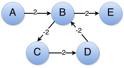
A Negative Cycle is a path V1 → V 2 → V3 → … Vk → V1 where the total sum of the edge weights in the path is negative. Consider the graph below –

bellman2

The path B → C → D is a negative cycle as the path’s total weight would be -2. So, the distance from A → B is 2, but if we circle the cycle once, we would get the distance as 0, if we circle once more, we would get -2. Like this we could keep on circling as much as we want to reduce the shortest distance. Hence the shortest distance to the vertex B, E becomes indeterminate.

So, we want Bellman Ford Algorithm to solve these two issues. We want it to compute the shortest path even for a graph with negative edges and negative cycles. The Bellman Ford will accurately compute the shortest path for a graph with negative edges but the algorithm fails for a graph with negative cycles. But, the algorithm can tell you if a negative cycle exists or not. If it exists the solution it puts up is incorrect, otherwise, the solution given by Bellman Ford Algorithm is perfect. This sounds fine because logically there will be no shortest paths for a graph with negative cycles.

Unlike the Dijkstra’s Algorithm where we had to use a priority queue, we will require no additional data structure to code Bellman Ford Algorithm. This makes writing the code much easier. And the algorithm is pretty straight-forward too. Take a look at the pseudo-code of the Bellman Ford Algorithm given below –

bellmanFord(G, s)
	for all edges in G(V)
		D(V) = INT_MAX
		parent[V] = -1

	D(s) = 0

	for i = 1 to |G(V)| - 1
		for each edge (u, v) in G(E)
			if edge can be Relaxed
				D(v) = D(u) + weight of edge (u, v)
				parent[v] = u

	for each edge in G(E)
		if edge can be Relaxed
			return false

	return true

You may not understand the pseudo-code at the first look, here’s a step-by-step representation of it –

  • Initialise the array which contains the shortest distances to infinity (a high integer value in the pseudo-code).
  • Initialise the parent array which contains the parent vertices in the shortest path to NULL (or -1 if it is an integer array).
  • Set the shortest distance of starting vertex to 0.
  • Explore all the edges, and see if you can relax them. If you can, relax the edge and proceed with the exploration.
  • Do the above operation |V| – 1 times.
  • After that, do another exploration on the graph checking all the edges if they can be relaxed. If they can be relaxed, you can a negative cycle in the graph. Hence, return false.
  • If the exploration gets finished successfully, the graph has no negative cycles and the data that you compute dis correct, so return true.

Now, what does exploring all the edges mean? If you are implementing the graph using an Adjacency List, it means to iterate over all the linked lists associated with all vertices. Now, what will be the sum of all the nodes in all Linked Lists in a given Adjacency List? Number of edges off course! So, we check all the edges from, edges of vertex 1 to vertex |V| in a linear manner. This whole operation takes O(|E|) time, which is repeated |V| – 1, so this part of the code takes O(|E||V|) time. Now, analyse the pseudo-code for a few minutes. Ask yourself how would you code this-ans-that. Now, when your mind is filled with the pseudo-code, look at the sketch below. The sketch below is sort of, “dry run” of the pseudo-code stated above –

bellman3

The above sketch is self-explanatory. I hope you understand how the iterations go. In a way it looks like a very ordinary algorithm, without any greedy steps or partitions or so. The Bellman Ford Algorithm is pretty easy to code too. If you can work hard for an hour or two I’m sure you can code this algorithm. It does not require any priority queue or other tools. All you need to code Bellman Ford Algorithm is the pseudo-code. The pseudo-code is very important. Keep looking at the pseudo-code again-and-again whenever you get a doubt. I have put my code below for a reference, it is a C++ code –

/*
 * Bellman-Ford Algorithm
 *
 * Authored by,
 * Vamsi Sangam
 */

#include <cstdio>
#include <cstdlib>
#include <climits>

using namespace std;

// This is used to construct
// the Adjacency List
struct node {
	int vertex, weight;
	struct node * next;
};

// This is used to construct the Shortest Paths to all
// vertices, as we cannot return multiple values,
// we use a struct
struct pathInfo {
	int vertex, distance, parent;
};

// Adds a new edge into the Adjacency List
// Follows Head Insertion for O(1) Insertion
struct node * add(struct node * head, int vertex, int weight)
{
	struct node * p = (struct node *) malloc(sizeof(struct node));

	p->vertex = vertex;
	p->weight = weight;
	p->next = head;

	return p;
}

// Bellman-Ford Algorithm which takes the Graph (adjacencyList[]), starting vertex (startVertex),
// and an empty array shortestDistances[] as input. It applies the algorithm and keeps filling values
// into shortestDistances[]. It returns true if there are no negative edges, and vice-versa.
bool bellmanFord(struct node * adjacencyList[], int vertices, int startVertex, struct pathInfo shortestDistances[])
{
	struct node * traverse;
	int i, j, k;

	// Initialisation
	for (i = 0; i <= vertices; ++i) {
		shortestDistances[i].vertex = i;
		shortestDistances[i].distance = INT_MAX;
		shortestDistances[i].parent = -1;
	}

	// Setting distance to source = 0
	shortestDistances[startVertex].parent = 0;
	shortestDistances[startVertex].distance = 0;

	// The Algorithm that computes Shortest Distances
	for (i = 1; i <= vertices - 1; ++i) {		// Runs 'vertices - 1' times = O(|V|)
		for (j = 1; j <= vertices; ++j) {		// Runs as many times as the edges = O(|E|)
			// The code ahead basically explores the whole of Adjcency List,
			// covering one edge once, so the runtime of the code in this
			// block is O(|E|)

			traverse = adjacencyList[j];

			while (traverse != NULL) {
				if (shortestDistances[j].distance == INT_MAX) {
					// Important...!
					traverse = traverse->next;
					continue;
				}

				// Checking for Relaxation
				if (traverse->weight + shortestDistances[j].distance < shortestDistances[traverse->vertex].distance) {
					// Relaxation
					shortestDistances[traverse->vertex].distance = traverse->weight + shortestDistances[j].distance;
					shortestDistances[traverse->vertex].parent = j;
				}

				traverse = traverse->next;
			}
		}
	}

	// Checking for Negative Cycles
	for (j = 1; j <= vertices; ++j) {
		traverse = adjacencyList[j];

		while (traverse != NULL) {
			// Checking for further relaxation
			if (traverse->weight + shortestDistances[j].distance < shortestDistances[traverse->vertex].distance) {
				// Negative Cycle found as further realxation is possible
				return false;
			}

			traverse = traverse->next;
		}
	}

	return true;
}

int main()
{
	int vertices, edges, i, j, v1, v2, weight;

	printf("Enter the Number of Vertices -\n");
	scanf("%d", &vertices);

	printf("Enter the Number of Edges -\n");
	scanf("%d", &edges);

	struct node * adjacency_list[vertices + 1];
	//Size is made (vertices + 1) to use the
	//array as 1-indexed, for simplicity

	//Must initialize your array
	for (i = 0; i <= vertices; ++i) {
		adjacency_list[i] = NULL;
	}
	printf("Enter the edges -\n\n");

	for (i = 1; i <= edges; ++i) {
		scanf("%d%d%d", &v1, &v2, &weight);
		adjacency_list[v1] = add(adjacency_list[v1], v2, weight);
	}

 	//Printing Adjacency List
	printf("\nAdjacency List -\n\n");
	for (i = 1; i <= vertices; ++i) {
		printf("adjacency_list[%d] -> ", i);

		struct node * temp = adjacency_list[i];

		while (temp != NULL) {
			printf("(%d, %d) -> ", temp->vertex, temp->weight);
			temp = temp->next;
		}

		printf("NULL\n");
	}

	struct pathInfo shortestDistances[vertices + 1];
	int startVertex;

	printf("\nEnter a Start Vertex -\n");
	scanf("%d", &startVertex);

	if (bellmanFord(adjacency_list, vertices, startVertex, shortestDistances)) {
		printf("No Negative Cycles exist in the Graph -\n");
	} else {
		printf("Negative Cycles exists in the Graph -\n");
		// The Bellman-Ford Algorithm does not work with negative cycles,
		// all it can do is merely detect them, so when a negative cycle
		// is detected, the shortestDistances array has wrong values
		return 0;
	}

	printf("\n\nVertex    Shortest Distance to Vertex %d     Parent Vertex-\n", startVertex);
	for (i = 1; i <= vertices; ++i) {
		printf("%d         %d                                 %d\n", i, shortestDistances[i].distance, shortestDistances[i].parent);
	}

	return 0;
}

If you have any doubts regarding the algorithm feel free to drop a comment. I’ll surely reply to them. I hope my post helped you in learning the Bellman Ford Algorithm. If it did, let me know by commenting ! Commenting is super easy if you are a Facebook, Twitter or a Google+ user…! So, don’t hesitate..! 😉 Keep practicing… Happy Coding…! 🙂

You may also like –

More in the Navigation Page ! →

Dijkstra’s Algorithm


Hello people…! In this post I will talk about one of the fastest single source shortest path algorithms, which is, the Dijkstra’s Algorithm. The Dijkstra’s Algorithm works on a weighted graph with non-negative edge weights and ultimately gives a Shortest Path Tree. It is a Greedy Algorithm, which sort of… mimics the working of Breadth First Search and Depth First Search. It is used in a number of day-to-day scenarios. It is used in network routing, to calculate the path from a network device A and B in a network which would have the maximum bandwidth. It could also be used by the GPS in a car to calculate the shortest path between two locations. The Dijkstra’s Algorithm can be modified to solve a lot of real world problems. So let’s get started…!

The Dijkstra’s Algorithm starts with a source vertex ‘s‘ and explores the whole graph. We will use the following elements to compute the shortest paths –

  • Priority Queue Q, implemented by a Min Binary Heap using C++ STL Vector.
  • Another set D, which keeps the record of the shortest paths from starting vertex s. Implemented using C++ STL Vector.

Just like the other graph search algorithms, Dijkstra’s Algorithm is best understood by listing out the algorithm in a step-by-step process –

  • The Initialisation –
  1. D(s), which is the shortest distance to s is set to 0. It is obvious as distance between source to itself is 0.
  2. For all the other vertices V, D(V) is set to infinity as we do not have a path yet to them, so we simply say that the distance to them is infinity.
  3. The Priority Queue Q, is constructed which is initially holds all the vertices of the Graph. Each vertex V will have the priority D(V).
  • The Algorithm –
  1. Now, pick up the first (or the minimum) element from the Priority Queue Q (which removes it from Q). For the first time, this operation would obviously give s.
  2. For all the vertices adjacent to s, i.e., for all vertices in adjacencyMatrix[s], check if the edge from s → v gives a shorter path. This is done by checking the following condition –

    if, D(s) + (weight of edge s → v) < D(v), we found a new shorter route, so update D(v)
    D(v) = D(s) + (weight of edge s → v)

  3. Now pick the next element from Q, and repeat the process until there are elements left in Q.

It might look like a long and cumbersome process, but this is actually a very smart technique. It’s okay if you don’t understand it in the first reading. Give another 3-4 readings and try to picture what is happening to the graph when you implement the algorithm, in your head. After you feel you have got a hang of the algorithm, look at the sketch below for complete understanding.

Dijkstra's Algorithm Step-by-Step

Dijkstra’s Algorithm Step-by-Step


The Dijkstra’s Algorithm is a little tricky. Many don’t understand it in the first attempt. In reference to the diagram above, I will give a step-by-step explanation for each graph marked with the number on top in purple.

  1. Firstly, initialize your components, the shortest distances array D, the priority queue Q, and starting vertex s. The distance from source to itself is zero. So, D(s) = 0, and the rest of the array is ∞ . The set of vertices V are inserted into the priority queue Q, with a priority D(V). Now, we start our algorithm by extracting (hence removing it from the priority queue) the minimum element from the priority queue. The minimum element in the priority queue will definitely be s (which is A here). Look at all the adjacent vertices of A. Vertices B, C, D are adjacent to A. We can go to B travelling the edge of weight 2, to C travelling an edge of weight 1, to D travelling an edge of weight 5. The values of D(B), D(C), D(D) are ∞ . We have found a new way of reaching them in 2, 1, 5 units respectively, which is less than ∞ , hence a shorter path. This is what the if-condition mentioned above does. So, we update the values of D(B), D(C), D(D) and the priorities of B, C, D, in the priority queue. With this we have finished processing the Vertex A.
  2. Now, the process continues to its next iteration and we extract the minimum element from the priority queue. The minimum element would be Vertex C which would be having a priority of 1. Now, look at all the adjacent vertices to C. There’s Vertex D. From C, the it would take 1 unit of distance to reach D. But to reach C in prior, you need 1 more unit of distance. So, if you go to D, via C, the total distance would be 2 units, which is less than the current value of shortest distance discovered to D, D(D) = 5. So, we reduce the value of D(D) to 2. This reduction is also called as “Relaxation”. With that we’re done with Vertex C.
  3. Now, the process continues to its next iteration and we extract the minimum element from the priority queue. Now, there are two minimum elements, B and D. You can go for anyone, it doesn’t matter. For now, we will go for Vertex D. From Vertex D, you can go to Vertex E, and Vertex F, with a total distance of 2 + 2 {D(D) + (weight of D → E)}, and 2 + 3. Which is less than ∞ , so D(E) becomes 4 and D(F) becomes 5. We’re done with Vertex D.
  4. Now, the process continues to its next iteration and we extract the minimum element from the priority queue. The minimum element in the priority queue is vertex B. From vertex B, you can reach vertex F in 2 + 1 units of distance, which is less than the current value of D(F), 5. So, we relax D(F) to 3. From vertex B, you can reach vertex D in 2 + 2 units of distance, which is more than the current value of D(D), 2. This route is not considered as it is clearly proven to be a longer route. With that we’re done with vertex B.
  5. Now, the process continues to its next iteration and we extract the minimum element from the priority queue. The minimum element in the priority queue is vertex E. From vertex E, you can reach vertex C in 4 + 4 units of distance, which is more than the current value of D(C), 1. This route is not considered as it is clearly proven to be a longer route. With that we’re done with vertex E.
  6. Now, the process continues to its next iteration and we extract the minimum element from the priority queue. The minimum element in the priority queue is vertex F. You cannot go to any other vertex from vertex F, so, we’re done with vertex F.
  7. With the removal of vertex F, our priority queue becomes empty. So, our algorithm is done…! You can simply return the array D to output the shortest paths.

Having got an idea about the overall working of the Dijkstra’s Algorithm, it’s time to look at the pseudo-code –

dijsktra(G, S)
	D(S) = 0
	Q = G(V)

	while (Q != NULL)
		u = extractMin(Q)
		for all V in adjacencyList[u]
			if (D(u) + weight of edge < D(V))
				D(V) = D(u) + weight of edge
				decreasePriority(Q, V)

In the pseudo-code, G is the input graph and S is the starting vertex. I hope you understand the pseudo-code. If you don’t, feel free to comment your doubts. Now, before we code Dijkstra’s Algorithm, we must first prepare a tool, which is the Priority Queue.

The Priority Queue

The Priority Queue is implemented by a number of data structures such as the Binary Heap, Binomial Heap, Fibonacci Heap, etc. The priority queue in my code is implemented by a Binary Heap. If you are not aware about the Binary Heap, you can refer to my post on Binary Heaps. But the implementation that we will do here is different from that in my post regarding the Binary Heap. The difference is that, here we will implement the Binary Heap using C++ STL Vector, not an array. This is because a heap is meant to grow, not remain of a fixed size, so we are using a data structure that can grow, a vector. Also, when we use a vector we can apply the same traversing techniques that we used in the case of an array. And, every element of our vector will be a Pair of two integers from the utility header file. The two integers represent vertex and weight, which is actually the shortest distances and this weight property will function as the priority to the elements. So, the vertices are placed in the priority queue based on their weight property. We will have to code the operations based on this weight property. Now the functionalities that we need from our priority queue are –

  • Insert – We will insert |V| elements into the Priority Queue.
  • Extract Min – We return the top-most element from the Binary Heap and delete it. Finally we make the neccessary
  • Decrease Priority – We decrease the priority of an element in the priority queue when we find a shorter path, as known as Relaxation.

If you know the working of the Binary Heap and have a little knowledge about the STL Library, you can code the Priority Queue in about 2-5 hours. You can keep referring to the internet of various functions and the syntaxes and any other doubts you have. Typing the code doesn’t take long, but debugging it and making it work takes the most time. That’s how you learn coding. Try your best, work on it for hours, if you don’t get it, take a break for 10-20 minutes… Come back and check my code below and try to figure out how close you were to getting it perfect…!

/*
 * Priority Queue implemented
 * by a Binary Heap using
 * C++ STL Vector, for
 * Dijkstra's Algorithm
 *
 * Authored by,
 * Vamsi Sangam
 */

#include <cstdio>
#include <vector>
#include <utility>

using namespace std;

// Inserts an element into the Queue
void enqueue(vector< pair<int, int> > * priorityQueue, pair<int, int> * entry)
{
	(*priorityQueue).push_back(*entry);

	int i = (*priorityQueue).size() - 1;
	pair<int, int> temp;

	while (i > 0) {
		if ((*priorityQueue)[(i - 1) / 2].second > (*priorityQueue)[i].second) {
			temp = (*priorityQueue)[(i - 1) / 2];
			(*priorityQueue)[(i - 1) / 2] = (*priorityQueue)[i];
			(*priorityQueue)[i] = temp;

			i = (i - 1) / 2;
		} else {
			break;
		}
	}
}

// Iterates over the Queue to return the index of the element
int findByKey(vector< pair<int, int> > * priorityQueue, pair<int, int> entry)
{
	int i;

	for (i = 0; i < (*priorityQueue).size(); ++i) {
		if ((*priorityQueue)[i].first == entry.first) {
			break;
		}
	}

	if (i != (*priorityQueue).size()) {
		return i;
	} else {
		return -1;
	}
}

// Decreases the priority of the element and makes neccessary adjustments
void decreasePriority(vector< pair<int, int> > * priorityQueue, int index, int newWeight)
{
	(*priorityQueue)[index].second = newWeight;

	int i = index;
	pair<int, int> temp;

	while (i > 0) {
		if ((*priorityQueue)[(i - 1) / 2].second > (*priorityQueue)[i].second) {
			temp = (*priorityQueue)[(i - 1) / 2];
			(*priorityQueue)[(i - 1) / 2] = (*priorityQueue)[i];
			(*priorityQueue)[i] = temp;

			i = (i - 1) / 2;
		} else {
			break;
		}
	}
}

// Returns the minimum element, deletes it and makes neccessary changes
pair<int, int> extractMin(vector< pair<int, int> > * priorityQueue)
{
	pair<int, int> min = (*priorityQueue)[0];
	pair<int, int> temp;

	// Swap first and last
	temp = (*priorityQueue)[0];
	(*priorityQueue)[0] = (*priorityQueue)[(*priorityQueue).size() - 1];
	(*priorityQueue)[(*priorityQueue).size() - 1] = temp;

	(*priorityQueue).pop_back();

	int i = 0;
	pair<int, int> parent;
	pair<int, int> rightChild;
	pair<int, int> leftChild;

	while (i < (*priorityQueue).size()) {
		parent = (*priorityQueue)[i];
		printf("Currently at - (%d, %d)\n", parent.first, parent.second);

		if (2 * (i + 1) < (*priorityQueue).size()) {
			// both children exist
			rightChild = (*priorityQueue)[2 * (i + 1)];
			leftChild = (*priorityQueue)[2 * (i + 1) - 1];

			if (parent.second < leftChild.second && parent.second < rightChild.second) {
				break;
			} else {
				if (leftChild.second < rightChild.second) {
					temp = (*priorityQueue)[2 * (i + 1) - 1];
					(*priorityQueue)[2 * (i + 1) - 1] = (*priorityQueue)[i];
					(*priorityQueue)[i] = temp;

					i = 2 * (i + 1) - 1;
				} else {
					temp = (*priorityQueue)[2 * (i + 1) - 1];
					(*priorityQueue)[2 * (i + 1) - 1] = (*priorityQueue)[i];
					(*priorityQueue)[i] = temp;

					i = 2 * (i + 1);
				}
			}
		} else if ((2 * (i + 1)) >= (*priorityQueue).size() && (2 * (i + 1) - 1) < (*priorityQueue).size()) {
			// only left child exists
			leftChild = (*priorityQueue)[2 * (i + 1) - 1];

			if (leftChild.second < parent.second) {
				temp = (*priorityQueue)[2 * (i + 1) - 1];
				(*priorityQueue)[2 * (i + 1) - 1] = (*priorityQueue)[i];
				(*priorityQueue)[i] = temp;
			}

			break;
		} else {
			// no more children exist
			break;
		}
	}

	return min;
}

int main()
{
	int n;

	printf("Enter the size -\n");
	scanf("%d", &n);

	int vertex, weight, i;
	vector< pair<int, int> > priorityQueue;
	pair<int, int> entry;

	for (i = 0; i < n; ++i) {
		scanf("%d%d", &vertex, &weight);
		entry = make_pair(vertex, weight);
		enqueue(&priorityQueue, &entry);
	}

	printf("\n\nThe Priority Queue (Interpret as Binary Heap) -\n");

	vector< pair<int, int> >::iterator itr = priorityQueue.begin();

	while (itr != priorityQueue.end()) {
		printf("(%d, %d) ", (*itr).first, (*itr).second);
		++itr;
	}
	printf("\n");

	pair<int, int> min = extractMin(&priorityQueue);
	printf("\n\nExtract Min returned = (%d, %d), The Queue -\n", min.first, min.second);
	itr = priorityQueue.begin();

	while (itr != priorityQueue.end()) {
		printf("(%d, %d) ", (*itr).first, (*itr).second);
		++itr;
	}
	printf("\n");

	decreasePriority(&priorityQueue, priorityQueue.size() - 1, 1);
	printf("\n\ndecreasePriority() used, The Queue -\n");
	itr = priorityQueue.begin();

	while (itr != priorityQueue.end()) {
		printf("(%d, %d) ", (*itr).first, (*itr).second);
		++itr;
	}
	printf("\n");

	return 0;
}

There are many other functionalities that a Priority Queue can give. But for now, we’ll need only these.

Joining the pieces

After you have your tool ready, you are all good to code Dijkstra’s Algorithm. Coding the Dijkstra’s Algorithm is easy but can go really weird. This is because you need to handle and co-ordinate many data structures at once. You’ll have to manage the adjacency list, the priority queue, the shortest distance array, and most importantly your loops…! You will surely end up spending more time in debugging the code, which is perfectly the right way of doing it. All throughout the coding, keep revising the step-by-step process explained above. If you don’t get it you, don’t fret, I put my code below. Before you look at my code, I would like to mention a few things –

  • We cannot have infinity in programming, so the shortest distances are initialised to the highest possible value in integer range, present in a macro, INT_MAX, in the header file climits.
  • The header file utility must be included to use pairs.
/* 
 * Dijkstra's Algorithm in C++
 * using Binary Heap as Priority
 * Queue implemented using 
 * C++ STL Vector
 *
 * Authored by,
 * Vamsi Sangam
 */

#include <cstdio>
#include <cstdlib>
#include <climits>
#include <vector>
#include <utility>

using namespace std;

// Our Vertex for Graph
struct node {
	int vertex, weight;
	struct node * next;
};

// To construct our Adjacency List
// Follows Head Insertion to give O(1) insertion
struct node * addEdge(struct node * head, int vertex, int weight)
{	 
	struct node * p = (struct node *) calloc(1, sizeof(struct node));
	
	p->vertex = vertex;
	p->weight = weight;
	p->next = head;
	
	return p;
}

// Adds vertices to the Priority Queue, Vertices a represented
// as pairs of vertex number and its shortest distance.
// This is logically a Binary Heap Insertion
void enqueue(vector< pair<int, int> > * priorityQueue, pair<int, int> * entry)
{
	(*priorityQueue).push_back(*entry);
	
	int i = (*priorityQueue).size() - 1;
	pair<int, int> temp;
	
	while (i > 0) {
		// Checking the priority of the parent, if greater, swap, else, we are done
		if ((*priorityQueue)[(i - 1) / 2].second > (*priorityQueue)[i].second) {
			temp = (*priorityQueue)[(i - 1) / 2];
			(*priorityQueue)[(i - 1) / 2] = (*priorityQueue)[i];
			(*priorityQueue)[i] = temp;
			
			i = (i - 1) / 2;
		} else {
			break;
		}
	}
}

// Finds for a Vertex in the Priority Queue and 
// returns its index as in its vector implementation
int findByKey(vector< pair<int, int> > * priorityQueue, pair<int, int> entry)
{
	int i;
	
	// Linear Search
	for (i = 0; i < (*priorityQueue).size(); ++i) {
		if ((*priorityQueue)[i].first == entry.first) {
			break;
		}
	}
	
	if (i != (*priorityQueue).size()) {
		return i;
	} else {
		return -1;
	}
}

// Decreases the priority of a given entry in the
// Priority Queue who's location is given by 'index'
// to 'newWeight' and re-arranges the Binary Heap
void decreasePriority(vector< pair<int, int> > * priorityQueue, int index, int newWeight)
{
	// Decreasing Priority
	(*priorityQueue)[index].second = newWeight;
	
	int i = index;
	pair<int, int> temp;
	
	// Adjusting the Binary Heap, similar re-arrangement as done in enqueue()
	while (i > 0) {
		if ((*priorityQueue)[(i - 1) / 2].second > (*priorityQueue)[i].second) {
			temp = (*priorityQueue)[(i - 1) / 2];
			(*priorityQueue)[(i - 1) / 2] = (*priorityQueue)[i];
			(*priorityQueue)[i] = temp;
			
			i = (i - 1) / 2;
		} else {
			break;
		}
	}
}

// Picks up the minimum element of the Priority Queue and re-arranges
// the Binary Heap and finally returns the Minimum Element picked.
// Functionally resembles Delete operation in Binary Heap, but additionally
// returns the deleted element which is the minimum element.
pair<int, int> extractMin(vector< pair<int, int> > * priorityQueue)
{
	pair<int, int> min = (*priorityQueue)[0];		// Min Element Stored
	pair<int, int> temp;
	
	// Swap first and last elements
	temp = (*priorityQueue)[0];
	(*priorityQueue)[0] = (*priorityQueue)[(*priorityQueue).size() - 1];
	(*priorityQueue)[(*priorityQueue).size() - 1] = temp;
	
	(*priorityQueue).pop_back();					// Deleted Min Element
	
	int i = 0;
	pair<int, int> parent;			// These three variables
	pair<int, int> rightChild;		// are for readability of
	pair<int, int> leftChild;		// the if conditions ahead
	
	while (i < (*priorityQueue).size()) {
		parent = (*priorityQueue)[i];
		
		if (2 * (i + 1) < (*priorityQueue).size()) {
			// both children exist
			rightChild = (*priorityQueue)[2 * (i + 1)];
			leftChild = (*priorityQueue)[2 * (i + 1) - 1];
			
			if (parent.second < leftChild.second && parent.second < rightChild.second) {
				// Parent has lesser priority than its children, so wer're done
				break;
			} else {
				if (leftChild.second < rightChild.second) {
					// Left-child has a lesser priority, so, swap
					temp = (*priorityQueue)[2 * (i + 1) - 1];
					(*priorityQueue)[2 * (i + 1) - 1] = (*priorityQueue)[i];
					(*priorityQueue)[i] = temp;
				
					i = 2 * (i + 1) - 1;
				} else {
					// Right-child has a lesser priority, so, swap
					temp = (*priorityQueue)[2 * (i + 1) - 1];
					(*priorityQueue)[2 * (i + 1) - 1] = (*priorityQueue)[i];
					(*priorityQueue)[i] = temp;
				
					i = 2 * (i + 1);
				}
			}
		} else if ((2 * (i + 1)) >= (*priorityQueue).size() && (2 * (i + 1) - 1) < (*priorityQueue).size()) {
			// only left child exists
			leftChild = (*priorityQueue)[2 * (i + 1) - 1];
			
			if (leftChild.second < parent.second) {
				// Left-child has a lesser priority, so, swap
				temp = (*priorityQueue)[2 * (i + 1) - 1];
				(*priorityQueue)[2 * (i + 1) - 1] = (*priorityQueue)[i];
				(*priorityQueue)[i] = temp;
			}
			
			break;
		} else {
			// no more children exist
			break;
		}
	}
	
	return min;
}

// The Dijkstra's Algorithm sub-routine which takes the Graph as Adjcaency List,
// number of vertices, a starting vertex, and an empty shortestDistances array as
// input and computest the shortest paths and fills them up in the shortestDistances array
void dijkstra(struct node * adjacencyList[], int vertices, int startVertex, pair<int, int> shortestDistances[])
{
	int i;
	
	// Initially no routes to vertices are know, so all are infinity,
	// here, we initialize to a very high integer value
	for (i = 0; i <= vertices; ++i) {
		shortestDistances[i].first = INT_MAX;
		shortestDistances[i].second = -1;
	}
	
	// Setting distance to source to zero
	shortestDistances[startVertex].first = 0;
	shortestDistances[startVertex].second = 0;
		
	struct node * trav;
	vector< pair<int, int> > priorityQueue;
	pair<int, int> min;
	
	// Making a the vertex that corresponds to the
	// 'startVertex' which will have a priority of zero
	// and we begin to intialise the Priority Queue
	pair<int, int> entry = make_pair(startVertex, 0);
	enqueue(&priorityQueue, &entry);
	
	// Initialising Priority Queue
	for (i = 1; i <= vertices; ++i) {
		if (i == startVertex) {
			continue;
		} else {
			// Priorities are set to a high integer value
			entry = make_pair(i, INT_MAX);
			enqueue(&priorityQueue, &entry);
		}
	}

	// We have the tools ready..! Let's roll...!!
	while (priorityQueue.size() != 0) {		// Untill there are vertices to be processed in Queue
		min = extractMin(&priorityQueue);	// Greedily process the nearest vertex
		
		trav = adjacencyList[min.first];	// Checking all the vertices adjacent to 'min'
		while (trav != NULL) {
			if (shortestDistances[trav->vertex].first > shortestDistances[min.first].first + trav->weight) {
				// We have discovered a new shortest route
				// Make the neccesary adjustments in data
				entry = make_pair(trav->vertex, trav->weight);
				
				int index = findByKey(&priorityQueue, entry);
				
				decreasePriority(&priorityQueue, index, trav->weight);
				shortestDistances[trav->vertex].first = shortestDistances[min.first].first + trav->weight;
				shortestDistances[trav->vertex].second = min.first;
			}
			
			trav = trav->next;
		}
	}
}

void PrintShortestPath(pair<int, int> shortestDistances[], int vertex, int startVertex)
{
	if (vertex == startVertex) {
		printf("%d ", startVertex);
		return;
	} else {
		PrintShortestPath(shortestDistances, shortestDistances[vertex].second, startVertex);
		printf("%d ", vertex);
	}
}

int main()
{
	int vertices, edges, i, j, v1, v2, w;
	
	printf("Enter the Number of Vertices -\n");
	scanf("%d", &vertices);
	
	printf("Enter the Number of Edges -\n");
	scanf("%d", &edges);
	
	struct node * adjacencyList[vertices + 1];
	//Size is made (vertices + 1) to use the
	//array as 1-indexed, for simplicity
	
	//Must initialize your array
	for (i = 0; i <= vertices; ++i) {
		adjacencyList[i] = NULL;
	}
	
	printf("\n");
	
	for (i = 1; i <= edges; ++i) {
		scanf("%d%d%d", &v1, &v2, &w);
		adjacencyList[v1] = addEdge(adjacencyList[v1], v2, w);
	}
 
 	//Printing Adjacency List
	printf("\nAdjacency List -\n\n");
	for (i = 1; i <= vertices; ++i) {
		printf("adjacencyList[%d] -> ", i);
		
		struct node * temp = adjacencyList[i];
		
		while (temp != NULL) {
			printf("%d(%d) -> ", temp->vertex, temp->weight);
			temp = temp->next;
		}
		
		printf("NULL\n");
	}
	
	int startVertex;
	
	printf("Choose a Starting Vertex -\n");
	scanf("%d", &startVertex);
	
	pair<int, int> shortestDistances[vertices + 1];
	// shortestDistances.first = shortest distance calculated
	// shortestDistances.second = parent node
	
	dijkstra(adjacencyList, vertices, startVertex, shortestDistances);
	
	printf("\n\nDijkstra's Algorithm Used - Shortest Paths from Vertex %d -\n", startVertex);
	for (i = 1; i <= vertices; ++i) {
		printf("Vertex %d, Distance = %d, Parent = %d\n", i, shortestDistances[i].first, shortestDistances[i].second);
	}
	printf("\n");
	
	PrintShortestPath(shortestDistances, vertices /* The Last Vertex */, startVertex);
	
	return 0;
}

This is the Dijkstra’s Algorithm. The code is well commented with explanation. If you don’t understand anything or if you have any doubts. Feel free to comment them. Now talking about the complexity of Dijkstra’s Algorithm. We perform |V| enqueue operations into the priority queue, which take O(log N), here, N is |V|, so this takes O(|V| log |V|). And at most |E| decrease priority operations which will take O(|V|) time. The extract-min is also called |V| times which will take O(|V| log |V|) time. So, the overall complexity of Dijkstra’s Algorithm we wrote is O(|V| log |V| + |E||V|). Dijkstra’s Algorithm can be improved by using a Fibonacci Heap as a Priority Queue, where the complexity reduces to O(|V| log |V| + |E|). But the Fibonacci Heap is an incredibly advanced and difficult data structure to code. We’ll talk about that implementation later.

I really hope my post has helped you in understanding the Dijkstra’s Algorithm. If it did, let me know by commenting. I tried my best to keep it as simple as possible. If you have any doubts, you can comment them too and I will surely reply to them. This algorithm is a particularly tough one. So, good luck… Keep practicing and… Happy Coding…! 🙂

You may also like –

More in the Navigation Page ! →

Depth First Search (DFS) Algorithm


Hello people…! In this post I will talk about the other Graph Search Algorithm, the Depth First Search (DFS). Depth First Search is different by nature from Breadth First Search. As the name suggests, “Depth”, we pick up a vertex S and see all the other vertices that can possibly reached by that vertex and we do that to all vertices in V. Depth First Search can be used to search over all the vertices, even for a disconnected graph. Breadth First Search can also do this, but DFS is more often used to do that. Depth First Search is used to solve puzzles! You can solve a given maze or even create your own maze by DFS. DFS is also used in Topological Sorting, which is the sorting of things according to a hierarchy. It is also used to tell if a cycle exists in a given graph. There are many other applications of DFS and you can do a whole lot of cool things with it. So, lets get started…!

The way the Depth First Search goes is really like solving a maze. When you see a maze in a newspaper or a magazine or anywhere else, the way you solve it is you take a path and go through it. If you find any junction or a crossroad, where you have a choice of paths to choose, you mark that junction, take up a path and traverse the whole route in your brain. If you see a dead end, you realize that this leads you now where so you come back to the junction you marked before and take up another path of the junction. See if that is also a dead end, else you continue to explore the, puzzle as this route contributes in reaching your destination. Well, at least that’s how I solve a maze. But… I hope you get the idea. You pick up a path and you explore it as much as possible. When you can’t travel any further and you haven’t yet reached your destination, you come back to the starting point and pick another path.

In code, you do this by recursion. Because of the very nature of recursion. Your recursion stack grows-grows and eventually becomes an empty stack. If you think for a while you can notice that the way of traversing which I told you above is logically covering only the vertices accessible from a given vertex S. Such traversal can be implemented using a single function that is recursive. But we want to explore the whole graph. So, we will use another function to do this for us. So, DFS is a two-functions thing. We will come back to the coding part later. Now, DFS too can be listed out in a step-by-step process –

  • For a given set of vertices V = {V1, V2,V3…}, start with V1, and explore all the vertices that can possibly be reached from V1.
  • Then go to the next vertex V2, if it hasn’t been visited, explore all the nodes reachable from V2, if not, go for V3.
  • Similarly, go on picking up all the vertices one-by-one and explore as much as possible if it wasn’t visited at all.

Now, how do you tell if a vertex wasn’t visited earlier…? If it has no parent vertex assigned. So what you have to do when you visit a node is –

  • Set the parent vertex of the current vertex to be the vertex from where you reached that vertex. We will use an array to assign parent vertices, which is initialised to -1, telling that the vertices were never visited.
  • When you are starting your exploration from a vertex, say, V1, we assign parent[V1] = 0, because it has no parent. If there is an edge from V1 to V2, we say, parent[V2] = V1.

Let’s look at an example and see how DFS really works –

dfs1

The working of DFS is pretty clear from the picture. Notice how we would assign the parent vertices to each vertex. Once we have visited all the vertices from a given initial vertex V1, we backtrack to V1. What do we really mean by this “backtrack” here is that the recursion control will gradually come back to the function that started explopring from V1. We will understand this once we put DFS in code. And one more thing, whenever we got a choice of going to two vertices from one vertex, we preferred going to the vertex with the greater number. Why is this…? This is because we will be following Head Insertion in our Adjacency Lists to have O(1) Insertion operation. Now, assuming that we insert the vertices from Vertex 1 to Vertex 10, the greater number vertices will end up being in front of the Linked Lists. Take a moment to understand this. Even if you don’t understand, it’s ok…! You will get the hang of it later. Why I really did that was to explain you the concept of Edge Classification.

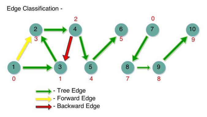
dfs2

As you can see there are three types of edges, in fact, there are 4 actually. They are –

  • Tree Edge – These are the edges through which we have traversed all the vertices of the graph by DFS. More clearly, these are the edges that represent the parent-child relationship. That is, the tree edge Vertex 1 → Vertex 3 says that, Vertex 1 is the parent of Vertex 3. Just like the parent-child relationship in a tree. Why this is called a “tree” edge is that it happens so that these edges together form a “tree”, or rather a “forest”.
  • Forward Edge – This is an edge which points from one vertex which is higher in the hierarchy of parent-child relationship to a vertex which is a descendant. Observe that Vertex 2 is a descendant of Vertex 1, so the edge Vertex 1 → Vertex 3, is a forward edge.
  • Backward Edge – This is the opposite of forward edge. It points from a descendant Vertex to an ancestor Vertex. In the above diagram, the edge, Vertex 4 → Vertex 3 is a backward edge.
  • Cross Edge – Every other edge is a cross edge. We don’t have a cross edge in the above diagram, but, a cross edge can arise when there is a edge between siblings, two vertices that have the same parent.

Cycle Detection – Using DFS, we can detect if there are any cycles in the given graph. How…? This is very simple. If there exists at least one backward edge, then the given graph will have cycles. Well, telling how many cycles would be there for given number of backward edges is a challenge. But the point is if there is a backward edge, there is a cycle. This is by the very definition of the Backward Edge. It is an edge from a descendant to an ancestor. If we have a backward edge, then there will surely be another path of tree edges from the ancestor to descendant, forming a cycle. The picture below should make things clear.

dfs3

But, how do we compute backward edges in code…? This is a little tricky. We could have a boolean array of size |V| which would hold the status of the vertex, whether it is in the recursion stack or not. If the vertex is in the recursion stack, it means that the vertex is indeed an ancestor. So, the edge will be a backward edge.

Now try to code the DFS, it is basically a recursion process. If you are good with recursion, I’m sure you can get this. Nonetheless, I have put my code below –

/* Depth First Search Algorithm
 * using Adjacency Lists
 *
 * Authored by,
 * Vamsi Sangam.
 */

#include <stdio.h>
#include <stdlib.h>

struct node {
	int val;
	struct node * next;
};

struct node * add(struct node * head, int num)
{
	/* We use Head Insertion for inserting vertices
	 * into Linked List for O(1) Insertion.
	 */

	struct node * p = (struct node *) malloc(sizeof(struct node));

	p->val = num;
	p->next = head;

	return p;
}

void depth_first_search_explore(struct node * list[], int parent[], int vertex, int status[])
{
	if (parent[vertex] != -1) {
		//un-visited vertex
		struct node * temp = list[vertex];
		status[vertex] = 1;

		//recursively visit all vertices accessible from this Vertex
		while (temp != NULL) {

			if (parent[temp->val] == -1) {
				parent[temp->val] = vertex;
				//We started exploring from Vertex -'vertex',
				//so the Vertex - temp->val, it's
				//parent should be our initial vertex

				depth_first_search_explore(list, parent, temp->val, status);
				//Then we recursively visit everything from the child vertex
			} else {
				//Checking if the edge is a Backward Edge
				if (status[temp->val] == 1) {
					printf("\n%d ---> %d is a Backward Edge\n", vertex, temp->val);
				}
			}

			temp = temp->next;
			//After finishing, move on to next Vertex adjacent to
			//Vertex - 'vertex'
		}

		status[vertex] = 0;
	}
}

void depth_first_search(struct node * list[], int length, int parent[], int status[])
{
	int i;

	for (i = 1; i <= length; ++i) {

		if (parent[i] == -1) {
			parent[i] = 0;
			//It is a completely un-visited vertex and we start
			//our DFS from here, so it has no parent, but just
			//to mark it that we visited this node, we assign 0

			depth_first_search_explore(list, parent, i, status);
			//By this we begin to explore all the vertices reachable
			//from Vertex i
		}
	}
}

int main()
{
	int vertices, edges, i, j, v1, v2;

	printf("Enter the Number of Vertices -\n");
	scanf("%d", &vertices);

	printf("Enter the Number of Edges -\n");
	scanf("%d", &edges);

	struct node * adjacency_list[vertices + 1];
	int parent[vertices + 1];
	int status[vertices + 1];
	//Size is made (vertices + 1) to use the
	//array as 1-indexed, for simplicity

	//Must initialize your array
	for (i = 0; i <= vertices; ++i) {
		adjacency_list[i] = NULL;
		parent[i] = -1;
		status[i] = 0;
	}

	printf("\n");

	for (i = 1; i <= edges; ++i) {
		scanf("%d%d", &v1, &v2);
		adjacency_list[v1] = add(adjacency_list[v1], v2);		//Adding edge v1 ------> v2
	}

 	//Printing Adjacency List
	printf("\nAdjacency List -\n\n");
	for (i = 1; i <= vertices; ++i) {
		printf("adjacency_list[%d] -> ", i);

		struct node * temp = adjacency_list[i];

		while (temp != NULL) {
			printf("%d -> ", temp->val);
			temp = temp->next;
		}

		printf("NULL\n");
	}

	depth_first_search(adjacency_list, vertices, parent, status);

	printf("\nParent Array -\n");
	for (i = 1; i <= vertices; ++i) {
		printf("Parent of Vertex %d = %d\n", i, parent[i]);
	}

	return 0;
}

The code above has an additional feature. It prints out the Backward Edges. This is done by the technique explained above, implemented using an integer array. I know it is a dirty way to use an integer array for this, it consumes way too much space. It really needs to be a Boolean array, because we use on two values, 0 and 1. But I wanted to keep my code strictly in C, so I used an integer array. This is the Depth First Search Algorithm. It has a time complexity of O(|V| + |E|), just like the Breadth First Search. This is because, we visit every vertex once, or you could say, twice, and we cover all the edges that AdjacencyList[Vi] has, for all ViV which takes O(|E|) time, which is actually the for loop in our depth_first_search_explore() function. DFS is not very difficult, you just need to have experienced hands in recursion. You might end up getting stuck with some bug. But it is worth spending time with the bugs because they make you think in the perfect direction. So if you are not getting the code, you just have to try harder. But if you are having any doubts, feel free to comment them…! Keep practicing… Happy Coding…! 🙂

You may also like –

More in the Navigation Page ! →

Snakes and Ladders Game Code


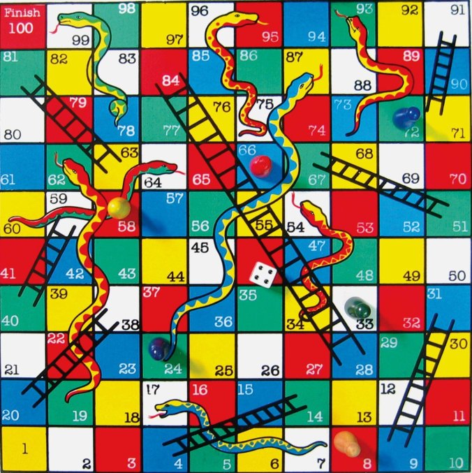
Hello people…! In this post I will explain you how to find the shortest path to win the Snakes and Ladder game by using the Breadth First Search (BFS) Algorithm. If you don’t know the algorithm, I suggest you read my post about it. Now, Graph Theory has many applications and I love working with things that have real-world applications, well, off course the other data structures too have their uses but the speciality of Graph Theory is its applications have the closest association with our day-to-day activities. And to show you this and to set an example on how the BFS is actually put into action, I am taking up the example of the very popular game, Snakes and Ladder. Now, this game needs no introduction. We all must have played it in our childhood. I will explain you… How by using Graphs and BFS we can find the Shortest Path to win the game, and, we will state that path and the number of moves of dice it takes too. Have a good look at the Snakes and Ladder board below, we will be using it as an example throughout this post.

snakes-and-ladders

You can see we can reach the finish block by an number of ways, but how do you find out the best…? More importantly, how do you put it as code…? That’s what we are going to do. Now, think of how you can represent the game board in terms of a Graph, by Graph I mean in terms of Vertices and Edges. Don’t be too hard on yourself… Just take the first 7 blocks and try working out on paper what would be the Edge and what would be the Vertices. If you ponder upon this, it is very easy to tell that the numbered blocks on the game board will be our Vertices, then, what will be the Edges…? This depends on how you can go from one block to another on rolling the dice. For now, forget about the ladders and the snakes, just draw the graph for a small portion of the board. It should look somewhat similar to what is in the picture below –

snake1

As you see we would have six ways to leave block 1, depending on the dice roll. Same would be the case for block 2, or, block 3, and so on. Now, there is a very important point to be noted here… Remember, this is Directed Graph…! Because, once you roll 5 and go to block 6, there’s no way to come back. So, the directions are important. Now, let us push up the complexity a bit by adding a ladder to our above sketch in block 6, think what would happen to the edges…?

snake2

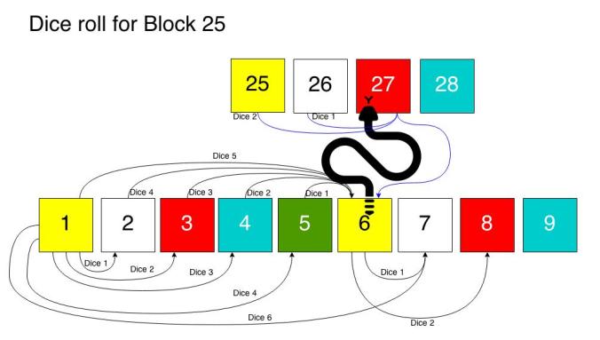
If you roll 5 from block 1 you will jump directly to block 27. So is for block 2 when you roll out 4, or, block 3 when you roll out 3 and so on. Now, “logically” speaking, the block 6 does not exists in our graph…! Think about the statement for a while. Whenever you reach block, you are directly jumping to block 27, you don’t stay there. Now, if you were constructing an Adjacency List for this graph…. In the list of adjacent vertices for Vertex 1, would you have Vertex 6 in the list, or Vertex 27…? Vertex 27 of course…! Being at Vertex 6 means being at Vertex 27…! That is why, our edge arrow did not end at Vertex 6… See it…? One more thing, in your Adjacency List, in the list of adjacent vertices for Vertex 6, what would you have…? Nothing…! Because you cannot come to a situation where you would have to stay on Vertex 6 and roll the dice. So the adjacent nodes list corresponding to Vertex 6 should be empty. These two things are very important, when you implement the Adjacency List for the Snake and Ladder board.

Same would be the case, if a snake was there at a block. Logically that block will not exist as a vertex in our adjacency list, and the corresponding edges must be removed. The only difference being that, the edge created due to a snake can lead you to a block of lower value.

snake3

We assume that getting caught by a snake is always unfavorable, and will not add to the progress of a short path. Just to get a better idea of the scenario of a ladder and snake, I have depicted what the Adjacency List would look like for the above two examples shown in the pictures.

snake4

That pic should really clarify all the confusion about the graph. If you still don’t get it, feel free to comment your query…! Now, what do we do once we have the Adjacency List ready…? We just call the Breadth First Search method on that list…! Wait… Really…?! That’s it…? Yes…! You see the hardest part here in solving the Snakes and Ladder by graphs is correctly determining what your Vertices and Edges are. Once you get that, all you have to do is the Breadth First Search in the resultant graph. Then you can get the shortest path from Vertex 1 to Vertex 100. Now, try getting the Adjacency Lit correct and simply call the BFS method. I’m sure you will succeed if you put in a little dedication. But for those who tried and failed. I have put my code below. Before you look at my code, there are a few logics I have used –

  • In the beginning of the program, I added all theSorry for the bad snip…! edges as though the Game Board had no snakes or ladders at all (these number of edges is what I printed), then, I removed the
    respective edges concerning the snakes and ladders one-by-one.
  • When a Vertex ‘n’ has a ladder or a snake, we are supposed to
    eplace the corresponding edges as I depicted in the pictures above, for that, I replaced the Vertex n‘s edge with the new value, in Vertices (n – 1), (n – 2), (n – 3), (n – 4), (n – 5), (n – 6). Because it is only in these vertices that you can find an edge of vertex n.
  • I put all this replacing stuff in a function replace() which takes the Linked List and searches for a value ‘num’ and replaces it with the value ‘replaced_num’ when it finds it.
  • I used an extra element in my array to make them 1 – index based.
  • The number of moves to complete the shortest path would be the level of the last vertex, Vertex 100. Why…?! Think about it for a minute and you’ll get it…!
  • I backtracked from Vertex 100, finding who it’s parent was, then, who the parent’s parent was and so on to find the path and finally printed it in reverse order.
/*
 * Snake and Ladder Shortest Path in C
 * using Adjacency List and
 * Breadth First Search.
 *
 * Authored by,
 * Vamsi Sangam
 */

#include <stdio.h>
#include <stdlib.h>

struct node {
	int val;
	struct node * next;
};

struct node * add(struct node * head, int num)
{
	struct node * p = (struct node *) malloc(sizeof(struct node));

	p->val = num;
	p->next = head;

	return p;
}

void breadth_first_search(struct node * list[], int vertices, int parent[], int level[])
{
	struct node * temp;
	int i, par, lev, flag = 1;

	lev = 0;
	level[1] = lev;

	while (flag) {
		flag = 0;
		for (i = 1; i <= vertices; ++i) {
			if (level[i] == lev) {
				flag = 1;
				temp = list[i];
				par = i;

				while (temp != NULL) {
					if (level[temp->val] != -1) {
						temp = temp->next;
						continue;
					}

					level[temp->val] = lev + 1;
					parent[temp->val] = par;
					temp = temp->next;
				}
			}
		}

		++lev;
	}
}

void replace(struct node * head, int num, int replaced_num)
{
	struct node * p = head;

	while (p->next != NULL) {
		if (p->val == num) {
			break;
		}

		p = p->next;
	}

	p->val = replaced_num;
}

int main()
{
	int vertices, edges, i, j, v1, v2;

	vertices = 100;		//For a 10X10 board
	edges = 0;			//Just to count the edges

	struct node * list[vertices + 1];

	int parent[vertices + 1];
	int level[vertices + 1];	

	for (i = 0; i <= vertices; ++i) {
		//Initialising our arrays
		list[i] = NULL;
		parent[i] = 0;
		level[i] = -1;
	}

	for (i = 1; i <= vertices; ++i) {
		for (j = 1; j <= 6 && j + i <= 100; ++j) {
			list[i] = add(list[i], i + j);
			++edges;
		}
	}

	printf("Edges added so far = %d\n", edges);

	int num_ladders, num_snakes;

	printf("Enter the Number of Ladders and Snakes -\n");
	scanf("%d%d", &num_ladders, &num_snakes);

	printf("Enter the Ladder Edges -\n");
	//Dealing with Ladder Edges
	for (i = 0; i < num_ladders; ++i) {
		scanf("%d%d", &v1, &v2);

		j = v1 - 6;

		if (j < 1) {
			j = 1;
		}

		for (; j < v1; ++j) {
			replace(list[j], v1, v2);
		}
	}

	printf("Enter the Snake Edges -\n");
	//Dealing with Snakes Edges
	for (i = 0; i < num_snakes; ++i) {
		scanf("%d%d", &v1, &v2);

		j = v1 - 6;

		if (j < 0) {
			j = 0;
		}

		for (; j < v1; ++j) {
			//Replacing Vertex value v1 by v2
			replace(list[j], v1, v2);
		}
	}

	//Printing Adjacency List
	printf("\nAdjacency List -\n");
	for (i = 1; i <= vertices; ++i) {
		printf("%d -> ", i);

		struct node * temp = list[i];

		while (temp != NULL) {
			printf("%d -> ", temp->val);
			temp = temp->next;
		}

		printf("NULL\n");
	}

	breadth_first_search(list, vertices, parent, level);
	printf("\nNumber of Moves required = %d\n", level[vertices]);

	/*Just a little mechanism to print the shortest path*/
	int path[level[vertices] + 1];

	j = 100;
	path[0] = j;

	for (i = 1; i <= level[vertices]; ++i) {
		path[i] = parent[j];
		j = parent[j];
	}

	printf("\nShortest Path -\n");
	for (i = level[vertices]; i >= 0; --i) {
		printf("%d -> ", path[i]);
	}
	printf("Finish...!\n");

	return 0;
}

You can think of extending this to a 20 ✗ 20 Snakes and Ladder board or an nn board. You just have to add n2 edges to the graph. Solving puzzles by Graph Theory is real fun. I hope this post helped you. If you have any doubts, feel free to comment them. Keep practicing… and… Happy Coding…! 🙂

You may also like –

More in the Navigation Page ! →

Breadth First Search (BFS) Algorithm


Hello people…! In this post I will explain one of the most widely used Graph Search Algorithms, the Breadth First Search (BFS) Algorithm. Once you have learned this, you would have gained a new weapon in your arsenal, and you can start solving good number of Graph Theory related competitive programming questions.

What we do in a BFS is a simple step-by-step process, which is –

  1. Start from a vertex S. Let this vertex be at, what is called…. “Level 0”.
  2. Find all the other vertices that are immediately accessible from this starting vertex S, i.e., they are only a single edge away (the adjacent vertices).
  3. Mark these adjacent vertices to be at “Level 1”.
  4. There will be a challenge that you might be coming back to the same vertex due to a loop or a ring in the graph. If this happens your BFS will take time. So, you will go only to those vertices who do not have their “Level” set to some value.
  5. Mark which is the parent vertex of the current vertex you’re at, i.e., the vertex from which you accessed the current vertex. Do this for all the vertices at Level 1.
  6. Now, find all those vertices that are a single edge away from all the vertices which are at “Level 1”. These new set of vertices will be at “Level 2”.
  7. Repeat this process until you run out of graph.

This might sound heavy… Well atleast it would sound heavy to me if I heard it for the first time…! Many questions may pop-up in your mind, like, “How are we gonna do all that…?!”. Well, for now, focus on the concept, we will talk about the code later. And remember, we are talking about an Undirected Graph here. We will talk about Directed Graphs later. To understand the above stated steps, examine the picture below –

Breadth First Search Algorithm - Step-by-Step

Breadth First Search Algorithm – Step-by-Step

The sketch clearly shows you how we explore the vertices adjacent to a vertex and mark their levels. If you have noticed, whenever there were two ways of accessing the same vertex from multiple vertices of the same Level, i.e., in the diagram, Vertex 3 was accessible from Vertex 2 and Vertex 8, we preferred its parent to be Vertex 8, the larger number. Why is that so…? We will learn that in a short moment.

The concepts that I wish to emphasize from the above picture are, how BFS can tell you the shortest path from a given vertex (the start vertex) to all the other vertices and the number of edges or, the “length of the path”, would be the Level of that Vertex itself. This is a very important feature of the BFS, you will understand this more clearly when I explain it with the help of an example in a different post.

Now, having got some knowledge about the BFS, it is a good thing to do an exercise on this topic to really get the flow going. Try applying BFS on the Graph given. All you have to do is to implement the step-by-step process and get that final figure which I got above. And make sure you label the Levels and Parents for each vertex in the end.

bfs2

Now, we come to the code part of the Breadth First Search, in C. We use the same Adjacency List that we used in our discussion of Graph Theory Basics. Coming back to our BFS discussion, the level of each vertex is stored in a separate array and so is the case for parent of each vertex. The three arrays are initialized to appropriate values. Now recall our step-by-step process that was stated earlier. Try to put that in terms of pseudocode and then proper code. Take a while to think how you would do that. If you could code it, you are marvelous…! 😀 … If not, don’t fret, I put my code below…!

/* ==========  ========== ========== ========= */
//         Breadth First Search (BFS)          //
//               Algorithm in C                //
//                                             //
//         Functions follow Pascal Case        //
//           Convention and Variables      	   //
//         follow Camel Case Convention        //
//                                             //
//            Author - Vamsi Sangam            //
//            Theory of Programming            //
/* ========== ========== ========== ========== */

#include <stdio.h>
#include <stdlib.h>

struct Edge {
    int vertex;
    struct Edge * next;
};

// Inserts Node to the Linked List by Head Insertion - O(1)
// Returns address of head which is the newly created node.
struct Edge * AddEdge(struct Edge * currentHead, int newVertex)
{
    struct Edge * newHead
				 = (struct Edge *) malloc(sizeof(struct Edge));

    newHead->vertex = newVertex;
    newHead->next = currentHead;

    return newHead;
}

void BreadthFirstSearch(
						struct Edge * adjacencyList[],
						int vertices,
						int parent[],
						int level[],
						int startVertex
					   )
{
    struct Edge * traverse;
    int i, par, lev, flag = 1;
    // 'lev' represents the level to be assigned
    // 'par' represents the parent to be assigned
    // 'flag' used to indicate if graph is exhausted

    lev = 0;
    level[startVertex] = lev;
    // We start at startVertex

    while (flag) {
        flag = 0;
        for (i = 1; i <= vertices; ++i) {
            if (level[i] == lev) {
                flag = 1;
                traverse = adjacencyList[i];
                par = i;

                while (traverse != NULL) {
                    if (level[traverse->vertex] != -1) {
                        traverse = traverse->next;
                        continue;
                    }

                    level[traverse->vertex] = lev + 1;
                    parent[traverse->vertex] = par;
                    traverse = traverse->next;
                }
            }
        }

        ++lev;
    }
}

int main()
{
    int vertices, edges, i, v1, v2;

    printf("Enter the Number of Vertices -\n");
    scanf("%d", &vertices);

    printf("\nEnter the Number of Edges -\n");
    scanf("%d", &edges);

    struct Edge * adjacencyList[vertices + 1];
    // Size is made (vertices + 1) to use the
    // array as 1-indexed, for simplicity

    int parent[vertices + 1];
    // Each element holds the Node value of its parent
    int level[vertices + 1];
    // Each element holds the Level value of that node

    // Must initialize your array
    for (i = 0; i <= vertices; ++i) {
        adjacencyList[i] = NULL;
        parent[i] = 0;
        level[i] = -1;
    }

    for (i = 1; i <= edges; ++i) {
        scanf("%d%d", &v1, &v2);

        // Adding edge v1 --> v2
        adjacencyList[v1] = AddEdge(adjacencyList[v1], v2);

		// Adding edge v2 --> v1
		// Remove this if you want a Directed Graph
        adjacencyList[v2] = AddEdge(adjacencyList[v2], v1);
    }

    // Printing Adjacency List
    printf("\nAdjacency List -\n\n");
    for (i = 1; i <= vertices; ++i) {
        printf("adjacencyList[%d] -> ", i);

        struct Edge * traverse = adjacencyList[i];

        while (traverse != NULL) {
            printf("%d -> ", traverse->vertex);
            traverse = traverse->next;
        }

        printf("NULL\n");
    }

    printf("\nEnter a Start Vertex - ");
    scanf("%d", &v1);

    BreadthFirstSearch(adjacencyList, vertices, parent, level, v1);

    // Printing Level and Parent Arrays
    printf("\nLevel and Parent Arrays -\n");
    for (i = 1; i <= vertices; ++i) {
        printf("Level of Vertex %d is %d, Parent is %d\n",
								  i, level[i], parent[i]);
    }

    return 0;
}

Try using the above example given as practice as the sample input to your code, so that you can easily compare the results. Now, the important point here is when we insert a vertex into the Adjacency List, we follow Head Insertion to get O(1) Insertion. What happens due to this is that, the Linked List will have numbers in the descending order.

So, when we are applying BFS for adjacent vertices of a given node, the Vertex with the higher number is met first. And then we explore starting by that higher numbered Vertex. This is why whenever we had a choice in approaching a vertex, we preferred approaching from the vertex which had the bigger number, why…? Due to Head Insertion…! If you had used Tail Insertion, this would be reversed.

Other Implementations of BFS

This is the overview of Breadth First Search Algorithm. It has a computational complexity of O(|V| + |E|), which is pretty fast. But why O(|V| + |E|)…? If you think about the algorithm a little bit, we cover all the |V| vertices level-by-level, checking all the |E| edges twice (for an Undirected Graph). Once the level is set for a subset of vertices we don’t visit them again. Put an itty-bitty thought into it and I’m sure you’ll get the idea…! 😉 … But, the code above runs slower than O(|V| + |E|)… To achieve the proper complexity we must use a Queue.

We can use BFS in the following scenarios –

  • Shortest Path or Quickest Path (if all edges have equal weight).
  • Finding the Length of Shortest Path between two Vertices.

With the knowledge of BFS you can start solving Graph Theory related problems. It really depends on your logic how you will apply the BFS to the given problem. And there is only one way to develop it… Practice…! So, keep practicing… Feel free to comment your doubts..! Commenting is super easy if you are a Facebook, Twitter or a Google+ user…! So, don’t hesitate..! 😉 … Happy Coding…! 🙂

Go to the Homepage →

Graph Theory Basics


Hello people…! In this post, I will talk about the basics of the Graph Data Structure. Its terminologies, types and implementations in C. Graphs are difficult to code, but they have the most interesting real-life applications. When you want to talk about the real-life applications of graphs, you just cannot resist talking about the Facebook’s Graph Search! Now, I don’t really know that algorithm, but it uses graphs to find out your closest friends, or any other associations you have with the other users.

Other applications include finding the shortest paths, and by shortest path, I mean in the “universal sense”, it could be the shortest path of a Traveling Salesman, or the shortest path to win Snake and Ladder or even the shortest way to solve the Rubik’s Cube…! Amazing, right…?! So, let’s get started…!

Graphs are much clear when defined in mathematical terms. A Graph G (V, E), consists of two sets,

  • Set of Vertices, V
  • Set of Edges, E

As the name suggest, V, is the set of vertices or, the set of all nodes in a given graph and E, is the set of all the edges between these nodes, or the associations between them. So, |V| denotes the number of nodes in a graph and |E| denotes the number of edges. Let us take up a small example to understand these terms –

Undirected and Directed Graph

Undirected and Directed Graph

As you can see, we have two types of graphs, Directed and Undirected Graphs. In Undirected Graphs,the direction for an edge is not defined. This is generally used to indicate that the edge is actually bi-directional in nature, i.e, one can go from V1 → V2, as well as from V2 → V1. This is used to represent the graph where the states (nodes) are re-doable, such as, in a Rubik’s Cube, you can go from one configuration of the cube to the other as well as the vice-versa.

The other type, the Directed Graph restricts the… “traversal”, if you say… to only one direction. For example, in the Snakes and Ladders game, you can play dice and go from Position 5 → Position 10, but you can’t roll the dice such that it gets you from Position 10 ← Position 5… That’s obvious…! So, it really depends on the requirement of the situation, which graph you choose. Generally, we only have to deal with graphs which are purely Directed or purely Undirected. We do not talk about the hybrid type. Some of the other type of graphs are shown below –

Types of Graphs

Types of Graphs

All the graphs which we have discussed till now are Simple Graphs, they do not contain any loops. The ones which do contain loops are Non-Simple. A given graph G can be drawn in any way as long as the sets V and E remain the same. Such a graph is shown in the figure. The same graph is just drawn differently, they both have the same set of vertices and edges. Such graphs are called as Isomorphic Graphs, as the name suggests “iso” means “same”, “morphic” means “shape”, the graphs which have the same shape.

All these Graphs are Connected Graphs, i.e., for any given pair of vertices V1 and V2 ∈ V, there always exists a path between these two vertices. The last graph is the Weighted Graph. Here, the edges are given “weights”. To understand a Weighted Graph, you can think of the vertices as cities and the edges as the distance between them (so they will have some value). You could be asked the shortest path between two cities. So in the context of a Weighted graph, the shortest path may not be the one with least edges. One must keep that in mind.

Now, we will look at the way the graphs are implemented. There are mainly two ways to implement graphs, they are –

  • Adjacency Matrix
  • Adjacency List

Adjacency Matrix

It is a very simple representation where we take a two-dimensional matrix of the size |V| × |V|, i.e., the declaration in C would look like,

int AdjacencyMatrix[V + 1][V + 1];

As the arrays are zero-indexed, we generally prefer to keep the sizes V + 1.Now, initially all the values would be zeroes. We put ‘1’ in an element of the two-dimensional array, AdjacencyMatrix[i][j], if there exists an edge between Vi → Vj. Remember, arrays are zero-indexed. Let us take an example to understand this,

Adjacency Matrix

Adjacency Matrix

I hope it is clear from the example, how we can represent the graph using an Adjacency Matrix. It is very easy to code. All you have to do is create a two-dimensional matrix and assign the values, so, I won’t post the code, but if you have any doubts regarding the code, feel free to comment them. The Adjacency Matrix has its pros and cons which we will discuss shortly.

Adjacency List

It is an array of pointers of size |V| + 1, where each pointer points to a linked list. The linked list holds the nodes which are adjacent to the ith vertex. By adjacent, we mean those vertices that can be accessed from ith node by making a single move. It is a little complex implementation if you are uncomfortable with linked lists. But it is this implementation that we will use for Graph Search Algorithms. This is because we can easily and efficiently know which of the vertices of V are neighbours of a given vertex. And that is what you want, if your are to do a Graph Search. Now, let us take an example to understand the concept of Adjacency Lists.

Adjacency List

Adjacency List

I hope the sketch has made it clear as to how we use the Adjacency List to implement a Graph. As I mentioned before, it is one of the most versatile implementations of the Graph Data Structure. Now, try to code the implementation in C, or any language you like. Please try this at least once by yourself so that you can get brain deep into the Graph Data Structure. It is only a linked list. And one more thing, don’t get confused between pointer-to-an-array and array-of-pointers…! So, if we put the value of |V| + 1 in a variable ‘vertices‘, now the declaration of our Adjacency List would be,

struct node * adjacency_list[vertices];

Remember this is an “array of pointers”, the declaration for “pointer to an array” would look like,

struct node (* adjcency_list)[vertices];

This is due to operator precedence. Some people make mistakes here, so, watch out! If you want to code in C++, we can have a vector where each element of the vector can hold another vector, so, the declaration would be, like,

list< vector<int> > adjacency_list;

Try to code for an hour or two… If you don’t get the code, it’s ok…! I’ve put my C code below. Those who got the code right… You are fabulous…! 😉 … But please take a minute to go through my code, I might have written a slightly better code than yours.

/* ==========  ========== ========== ========= */
//          Adjacency List Graph Data          //
//          Structure Implementation           //
//           in C using Linked List            //
//                                             //
//         Functions follow Pascal Case        //
//           Convention and Variables      	   //
//         follow Camel Case Convention        //
//                                             //
//            Author - Vamsi Sangam            //
//            Theory of Programming            //
/* ========== ========== ========== ========== */
 
#include <stdio.h>
#include <stdlib.h>
 
struct Edge {
    int vertex;
    struct Edge * next;
};

// Inserts Node to the Linked List by Head Insertion - O(1)
// Returns address of head which is the newly created node.
struct Edge * AddEdge(struct Edge * currentHead, int newVertex)
{
    struct Edge * newHead 
				 = (struct Edge *) malloc(sizeof(struct Edge));
 
    newHead->vertex = newVertex;
    newHead->next = currentHead;
 
    return newHead;
}

int main()
{
    int vertices, edges, i, v1, v2;
 
    printf("Enter the Number of Vertices -\n");
    scanf("%d", &vertices);
 
    printf("\nEnter the Number of Edges -\n");
    scanf("%d", &edges);
 
    struct Edge * adjacencyList[vertices + 1];
    // Size is made (vertices + 1) to use the
    // array as 1-indexed, for simplicity
 
    // Must initialize your array
    for (i = 0; i <= vertices; ++i) {
        adjacencyList[i] = NULL;
    }
 
    for (i = 1; i <= edges; ++i) {
        scanf("%d%d", &v1, &v2);
        
        // Adding edge v1 --> v2
        adjacencyList[v1] = AddEdge(adjacencyList[v1], v2);
		
		// Adding edge v2 --> v1
		// Remove this if you want a Directed Graph
        adjacencyList[v2] = AddEdge(adjacencyList[v2], v1);
    }
 
    // Printing Adjacency List
    printf("\nAdjacency List -\n\n");
    for (i = 1; i <= vertices; ++i) {
        printf("adjacencyList[%d] -> ", i);
 
        struct Edge * traverse = adjacencyList[i];
 
        while (traverse != NULL) {
            printf("%d -> ", traverse->vertex);
            traverse = traverse->next;
        }
 
        printf("NULL\n");
    }
 
    return 0;
}

Other implementations of Adjacency List

Comparison between Adjacency Matrix and Adjacency List

Adjacency Matrix Adjacency List
For a Directed Graph, it consumes O(|V|2) space which is often under-utilized in the implementation. For an Undirected Graph also, it consumes O(|V|2) space which is also under-utilized as the generated matrix is symmetric about diagonal and values just repeat. For a Directed Graph it consumes O(|V| + |E|) space which is less, and is utilized optimally. For an Undirected Graph it consumes O(|V| + 2 ✗ |E|) space, which is O(|V| + |E|), which is less.
As the memory allocation is contiguous, data access is slightly faster. It is basically a Linked List, so memory allocation is not contiguous, hence traversal is slow as as compared to the traversal in an array. However, this can be eliminated if we use a Vector of C++ STL Library in the place of the Linked List. But C++ STL Vector is not recommended for graphs that keep growing.
Inserting an edge takes O(1) time, i.e., constant time. Therefore, inserting |E| edges take O(|E|) time, as direct access is available. Inserting an edge can take O(|E|) in the worst case, which is, there is an edge between every pair of vertices, one must traverse the whole Linked List over-and-over causing insertion of |E| nodes to take O(|E|2) time. However, if one follows Head Insertion, inserting a node will take O(1) time, and inserting |E| nodes will take O(|E|) time.
Deleting an edge is very simple, we just set the corresponding element value to 0, which takes O(1) time. Deleting an edge is time-taking as, one would have to traverse the Linked List, which is slow (non-contiguous). In the worst case, it takes O(|E|) time.


With the knowledge of Adjacency Matrix and Adjacency List alone you won’t be able to do the competitive programming questions, because you do not know how to explore your graph to get the desired result. For this, you need to know the Breadth First Search (BFS) Algorithm and the Depth First Search (DFS) Algorithm. This post is only to give an introduction. Feel free to comment your doubts..! Commenting is super easy if you are a Facebook, Twitter or a Google+ user…! So, don’t hesitate..! 😉 … Keep practising…. Happy Coding…! 🙂